Методи компіляції для схем симуляції гамільтоніана
Оцінка використання: менше 1 хвилини на процесорі IBM Heron (ПРИМІТКА: це лише оцінка. Твій час може відрізнятися.)
Результати навчання
Після завершення цього підручника ти зрозумієш:
- Як використовувати транспілер Qiskit з SABRE для оптимізації компонування та маршрутизації
- Як використовувати транспілер з підтримкою AI для розширеної оптимізації схем
- Як використовувати плагін Rustiq для синтезу операцій
PauliEvolutionGateв схемах симуляції гамільтоніана - Як виконувати порівняльний аналіз методів компіляції за двоквітною глибиною, загальною кількістю гейтів та часом виконання
Передумови
Радимо ознайомитися з такими темами перед початком цього підручника:
Передмова
Компіляція квантових схем перетворює високорівневий квантовий алгоритм на фізичну схему, яка відповідає обмеженням цільового апаратного забезпечення. Ефективна компіляція може суттєво зменшити глибину схеми та кількість гейтів, що безпосередньо впливає на якість результатів на квантових пристроях найближчого часу.
Цей підручник порівнює три методи компіляції на схемах симуляції гамільтоніана, побудованих за допомогою PauliEvolutionGate. Ці схеми моделюють попарні взаємодії між квітами (такі як члени , та ) і широко використовуються у квантовій хімії, фізиці конденсованого стану та матеріалознавстві.
Схеми для порівняльного аналізу взяті з колекції Hamlib, доступ до якої здійснюється через репозиторій Benchpress. Hamlib надає стандартизований набір репрезентативних гамільтоніанів, що дозволяє порівнювати стратегії компіляції на реалістичних задачах симуляції.
Огляд методів компіляції
Транспілер Qiskit з SABRE
Транспілер Qiskit використовує алгоритм SABRE (SWAP-based BidiREctional heuristic search) для оптимізації компонування та маршрутизації схем. SABRE зосереджується на мінімізації гейтів SWAP та їхнього впливу на глибину схеми, дотримуючись обмежень зв'язності апаратного забезпечення. Це метод загального призначення, який забезпечує гарний баланс між продуктивністю та часом компіляції. Для отримання додаткової інформації дивись [1]. Переваги та дослідження параметрів SABRE детально розглядаються в окремому підручнику.
Транспілер з підтримкою AI
Транспілер з підтримкою AI використовує машинне навчання для прогнозування оптимальних стратегій транспіляції шляхом аналізу шаблонів у структурі схеми та обмежень апаратного забезпечення. Він також може застосовувати прохід AIPauliNetworkSynthesis, який націлений на схеми мережі Паулі з використанням підходу синтезу на основі навчання з підкріпленням. Для отримання додаткової інформації дивись [2] та [3].
Плагін Rustiq
Плагін Rustiq надає розширені техніки синтезу спеціально для операцій PauliEvolutionGate, які представляють обертання Паулі, що зазвичай використовуються в троттеризованій динаміці. Він розроблений для отримання декомпозицій схем з малою глибиною для задач симуляції гамільтоніана. Для отримання додаткової інформації дивись [4].
Ключові метрики
Ми порівнюємо три методи за такими метриками:
- Двоквітна глибина: Глибина схеми з урахуванням лише двоквітних гейтів. Це часто є вузьким місцем для точності на реальному апаратному забезпеченні.
- Розмір схеми (загальна кількість гейтів): Загальна кількість гейтів у транспільованій схемі.
- Час виконання: Реальний час транспіляції.
Вимоги
Перед початком цього підручника переконайся, що у тебе встановлено таке:
- Qiskit SDK v2.0 або новіше, з підтримкою візуалізації
- Qiskit Runtime v0.22 або новіше (
pip install qiskit-ibm-runtime) - Qiskit Aer (
pip install qiskit-aer) - Qiskit IBM Transpiler (
pip install qiskit-ibm-transpiler) - Qiskit AI Transpiler local mode (
pip install qiskit_ibm_ai_local_transpiler) - Networkx (
pip install networkx)
Налаштування
# Added by doQumentation — required packages for this notebook
!pip install -q matplotlib numpy qiskit qiskit-aer qiskit-ibm-runtime qiskit-ibm-transpiler requests scipy
from qiskit.circuit import QuantumCircuit
from qiskit_ibm_runtime import QiskitRuntimeService, SamplerV2
from qiskit.circuit.library import PauliEvolutionGate
from qiskit_ibm_transpiler import generate_ai_pass_manager
from qiskit.quantum_info import SparsePauliOp
from qiskit.transpiler.preset_passmanagers import generate_preset_pass_manager
from qiskit.transpiler.passes.synthesis.high_level_synthesis import HLSConfig
from qiskit_aer import AerSimulator
from qiskit_aer.noise import NoiseModel, depolarizing_error
from collections import Counter
from statistics import mean, stdev
from scipy.sparse import SparseEfficiencyWarning
import time
import warnings
import matplotlib.pyplot as plt
import matplotlib.ticker as ticker
import numpy as np
import json
import requests
import logging

# Suppress noisy loggers and warnings
logging.getLogger(
    "qiskit_ibm_transpiler.wrappers.ai_local_synthesis"
).setLevel(logging.ERROR)
warnings.filterwarnings("ignore", category=FutureWarning)
warnings.filterwarnings("ignore", category=SparseEfficiencyWarning)

seed = 42  # Seed for reproducibility
Підключення до бекенду
Вибери бекенд, який буде використовуватися як для малого, так і для великого масштабу прикладів. Бекенд визначає карту зв'язків та базові гейти, на які орієнтується транспілер.
# QiskitRuntimeService.save_account(channel="ibm_quantum_platform",
# token="<YOUR-API-KEY>", overwrite=True, set_as_default=True)
service = QiskitRuntimeService(channel="ibm_quantum_platform")
backend = service.least_busy(operational=True, simulator=False)
print(f"Using backend: {backend.name}")
Using backend: ibm_pittsburgh
Визначення менеджерів проходів
Налаштуй три методи компіляції.
# SABRE pass manager (Qiskit default at optimization level 3)
pm_sabre = generate_preset_pass_manager(
    optimization_level=3, backend=backend, seed_transpiler=seed
)
# AI transpiler pass manager (local mode)
pm_ai = generate_ai_pass_manager(
    backend=backend, optimization_level=3, ai_optimization_level=3
)
Fetching 127 files: 0%| | 0/127 [00:00<?, ?it/s]
# Rustiq pass manager for PauliEvolutionGate synthesis
hls_config = HLSConfig(
    PauliEvolution=[
        (
            "rustiq",
            {
                "nshuffles": 400,
                "upto_phase": True,
                "fix_clifford": True,
                "preserve_order": False,
                "metric": "depth",
            },
        )
    ]
)
pm_rustiq = generate_preset_pass_manager(
    optimization_level=3,
    backend=backend,
    hls_config=hls_config,
    seed_transpiler=seed,
)
Визначення допоміжних функцій
Наступна функція транспілює список схем за допомогою заданого менеджера проходів і записує ключові метрики (двоквітна глибина, розмір схеми та час виконання) для кожної схеми.
def capture_transpilation_metrics(
    results, pass_manager, circuits, method_name
):
    """
    Transpile circuits and append one metrics record per circuit to
    ``results``.

    Args:
        results (list): List of dicts to append the metrics records to.
        pass_manager: Pass manager used for transpilation.
        circuits (list): List of quantum circuits to transpile.
        method_name (str): Name of the transpilation method.

    Returns:
        list: List of transpiled circuits.
    """
    transpiled_circuits = []

    for i, qc in enumerate(circuits):
        start_time = time.time()
        transpiled_qc = pass_manager.run(qc)
        end_time = time.time()

        # Decompose swaps for consistency across methods
        transpiled_qc = transpiled_qc.decompose(gates_to_decompose=["swap"])

        transpilation_time = end_time - start_time
        two_qubit_depth = transpiled_qc.depth(
            lambda x: x.operation.num_qubits == 2
        )
        circuit_size = transpiled_qc.size()

        results.append(
            {
                "method": method_name,
                "qc_name": qc.name,
                "qc_index": i,
                "num_qubits": qc.num_qubits,
                "two_qubit_depth": two_qubit_depth,
                "size": circuit_size,
                "runtime": transpilation_time,
            }
        )
        transpiled_circuits.append(transpiled_qc)
        print(
            f"[{method_name}] Circuit {i} ({qc.name}): "
            f"2Q depth={two_qubit_depth}, size={circuit_size}, "
            f"time={transpilation_time:.2f}s"
        )

    return transpiled_circuits
def _method_order(results):
    """Return the distinct method names in their first-seen order."""
    order = []
    for r in results:
        if r["method"] not in order:
            order.append(r["method"])
    return order

def print_summary_table(results):
    """
    Print the mean and standard deviation of each metric per compilation
    method, followed by the mean percent improvement relative to SABRE.
    """
    metrics = [
        ("two_qubit_depth", "2Q Depth"),
        ("size", "Gate Count"),
        ("runtime", "Runtime (s)"),
    ]
    methods = _method_order(results)
    by_method = {m: [r for r in results if r["method"] == m] for m in methods}
    sabre_by_index = {r["qc_index"]: r for r in by_method.get("SABRE", [])}

    col_w = 22
    name_w = max(len(m) for m in methods)
    header = f"{'Method':<{name_w}}" + "".join(
        f"  {label:>{col_w}}" for _, label in metrics
    )

    print("Mean +/- std per compilation method")
    print(header)
    print("-" * len(header))
    for method in methods:
        cells = []
        for key, _ in metrics:
            values = [r[key] for r in by_method[method]]
            std = stdev(values) if len(values) > 1 else 0.0
            cells.append(f"{mean(values):,.1f} +/- {std:,.1f}")
        print(
            f"{method:<{name_w}}" + "".join(f"  {c:>{col_w}}" for c in cells)
        )

    others = [m for m in methods if m != "SABRE"]
    if others and sabre_by_index:
        print()
        print("Mean % improvement vs SABRE (positive = better than SABRE)")
        print(header)
        print("-" * len(header))
        for method in others:
            cells = []
            for key, _ in metrics:
                pct = [
                    (sabre_by_index[r["qc_index"]][key] - r[key])
                    / sabre_by_index[r["qc_index"]][key]
                    * 100
                    for r in by_method[method]
                    if sabre_by_index.get(r["qc_index"])
                    and sabre_by_index[r["qc_index"]][key]
                ]
                if pct:
                    std = stdev(pct) if len(pct) > 1 else 0.0
                    cells.append(f"{mean(pct):+.1f}% +/- {std:.1f}%")
                else:
                    cells.append("n/a")
            print(
                f"{method:<{name_w}}"
                + "".join(f"  {c:>{col_w}}" for c in cells)
            )
def print_per_circuit_comparison(results, num_rows=5):
    """
    Print a per-metric comparison of the compilation methods for the
    first ``num_rows`` circuits (sorted by qubit count). The best
    (lowest) value for each metric is marked with an asterisk.
    """
    metrics = [
        ("two_qubit_depth", "2Q Depth"),
        ("size", "Gate Count"),
        ("runtime", "Runtime (s)"),
    ]
    methods = _method_order(results)

    by_index = {}
    for r in results:
        by_index.setdefault(r["qc_index"], {})[r["method"]] = r
    ordered = sorted(
        by_index.items(),
        key=lambda kv: (next(iter(kv[1].values()))["num_qubits"], kv[0]),
    )[:num_rows]

    for key, label in metrics:
        print(f"{label} (first {num_rows} circuits by qubit count); * = best")
        header = f"{'Idx':>3}  {'Circuit':<16} {'Q':>3}" + "".join(
            f"{m:>9}" for m in methods
        )
        print(header)
        print("-" * len(header))
        for idx, method_map in ordered:
            any_record = next(iter(method_map.values()))
            present = {
                m: method_map[m][key] for m in methods if m in method_map
            }
            best = min(present.values())
            line = (
                f"{idx:>3}  {any_record['qc_name'][:16]:<16} "
                f"{any_record['num_qubits']:>3}"
            )
            for m in methods:
                value = method_map[m][key]
                text = f"{value:.2f}" if key == "runtime" else f"{int(value)}"
                if value == best:
                    text += "*"
                line += f"{text:>9}"
            print(line)
        print()
Завантаження схем гамільтоніана з Hamlib
Ми завантажуємо репрезентативний набір гамільтоніанів з репозиторію Benchpress та будуємо схеми PauliEvolutionGate. Схеми, що перевищують кількість квітів бекенду, видаляються разом зі схемами, розкладений розмір яких перевищує 1500 гейтів (щоб час транспіляції залишався розумним).
# Obtain the Hamiltonian JSON from the benchpress repository
url = "https://raw.githubusercontent.com/Qiskit/benchpress/e7b29ef7be4cc0d70237b8fdc03edbd698908eff/benchpress/hamiltonian/hamlib/100_representative.json"
response = requests.get(url)
response.raise_for_status()
ham_records = json.loads(response.text)

# Remove circuits that are too large for the backend
ham_records = [
    h for h in ham_records if h["ham_qubits"] <= backend.num_qubits
]

# Build PauliEvolutionGate circuits
qc_ham_list = []
for h in ham_records:
    terms = h["ham_hamlib_hamiltonian_terms"]
    coeff = h["ham_hamlib_hamiltonian_coefficients"]
    num_qubits = h["ham_qubits"]
    name = h["ham_problem"]

    evo_gate = PauliEvolutionGate(SparsePauliOp(terms, coeff))
    qc = QuantumCircuit(num_qubits)
    qc.name = name
    qc.append(evo_gate, range(num_qubits))
    qc_ham_list.append(qc)

# Remove circuits whose decomposed size exceeds 1500 gates so that transpilation completes in a reasonable time frame
qc_ham_list = [qc for qc in qc_ham_list if qc.decompose().size() <= 1500]

print(f"Total Hamiltonian circuits loaded: {len(qc_ham_list)}")
print(
    f"Qubit range: {min(qc.num_qubits for qc in qc_ham_list)} to {max(qc.num_qubits for qc in qc_ham_list)}"
)
Total Hamiltonian circuits loaded: 42
Qubit range: 2 to 112
Розділи схеми на малий масштаб (менше 20 квітів) та великий масштаб (20 або більше квітів).
qc_small = [qc for qc in qc_ham_list if qc.num_qubits < 20]
qc_large = [qc for qc in qc_ham_list if qc.num_qubits >= 20]

print(f"Small-scale circuits (<20 qubits): {len(qc_small)}")
print(f"Large-scale circuits (>=20 qubits): {len(qc_large)}")
Small-scale circuits (<20 qubits): 20
Large-scale circuits (>=20 qubits): 22
Попередній перегляд однієї малої схеми гамільтоніана перед транспіляцією.
# We decompose the circuit here, otherwise it would just be a PauliEvolutionGate box,
# which isn't very informative to look at!
qc_small[0].decompose().draw("mpl", fold=-1)

Приклад малого масштабу
У цьому розділі ми порівнюємо три методи компіляції на схемах гамільтоніана з менш ніж 20 квітами. Ці схеми транспілюються швидко і дають чітке уявлення про те, як кожен метод обробляє схеми помірної складності.
Крок 1: Відобрази класичні входи на квантову задачу
Кожен гамільтоніан закодований як схема PauliEvolutionGate. Схеми вже були побудовані в розділі налаштування з даних бенчмарку Hamlib.
Крок 2: Оптимізуй задачу для виконання на квантовому апаратному забезпеченні
Ми транспілюємо всі малі схеми за допомогою кожного з трьох менеджерів проходів, а потім збираємо метрики.
results_small = []

tqc_sabre_small = capture_transpilation_metrics(
    results_small, pm_sabre, qc_small, "SABRE"
)
tqc_ai_small = capture_transpilation_metrics(
    results_small, pm_ai, qc_small, "AI"
)
tqc_rustiq_small = capture_transpilation_metrics(
    results_small, pm_rustiq, qc_small, "Rustiq"
)
[SABRE] Circuit 0 (all-vib-bh): 2Q depth=3, size=30, time=2.09s
[SABRE] Circuit 1 (all-vib-c2h): 2Q depth=18, size=111, time=0.01s
[SABRE] Circuit 2 (all-vib-o3): 2Q depth=6, size=58, time=0.00s
[SABRE] Circuit 3 (all-vib-c2h): 2Q depth=2, size=37, time=0.01s
[SABRE] Circuit 4 (graph-gnp_k-2): 2Q depth=24, size=126, time=0.01s
[SABRE] Circuit 5 (LiH): 2Q depth=66, size=285, time=0.01s
[SABRE] Circuit 6 (all-vib-fccf): 2Q depth=66, size=339, time=0.01s
[SABRE] Circuit 7 (all-vib-ch2): 2Q depth=88, size=413, time=0.01s
[SABRE] Circuit 8 (all-vib-f2): 2Q depth=180, size=1000, time=0.02s
[SABRE] Circuit 9 (all-vib-bhf2): 2Q depth=18, size=223, time=0.03s
[SABRE] Circuit 10 (graph-gnp_k-4): 2Q depth=122, size=675, time=0.02s
[SABRE] Circuit 11 (Be2): 2Q depth=343, size=1628, time=0.03s
[SABRE] Circuit 12 (all-vib-fccf): 2Q depth=14, size=134, time=0.00s
[SABRE] Circuit 13 (uf20-ham): 2Q depth=50, size=341, time=0.01s
[SABRE] Circuit 14 (TSP_Ncity-4): 2Q depth=118, size=615, time=0.01s
[SABRE] Circuit 15 (graph-complete_bipart): 2Q depth=232, size=1420, time=0.03s
[SABRE] Circuit 16 (all-vib-cyclo_propene): 2Q depth=18, size=354, time=0.93s
[SABRE] Circuit 17 (all-vib-hno): 2Q depth=6, size=174, time=0.14s
[SABRE] Circuit 18 (all-vib-fccf): 2Q depth=30, size=286, time=0.01s
[SABRE] Circuit 19 (tfim): 2Q depth=31, size=232, time=0.03s
[AI] Circuit 0 (all-vib-bh): 2Q depth=3, size=30, time=0.01s
Fetching 4 files: 0%| | 0/4 [00:00<?, ?it/s]
[AI] Circuit 1 (all-vib-c2h): 2Q depth=18, size=101, time=0.18s
[AI] Circuit 2 (all-vib-o3): 2Q depth=6, size=58, time=0.01s
[AI] Circuit 3 (all-vib-c2h): 2Q depth=2, size=37, time=0.01s
[AI] Circuit 4 (graph-gnp_k-2): 2Q depth=24, size=133, time=0.07s
[AI] Circuit 5 (LiH): 2Q depth=62, size=267, time=8.00s
[AI] Circuit 6 (all-vib-fccf): 2Q depth=65, size=300, time=0.18s
[AI] Circuit 7 (all-vib-ch2): 2Q depth=79, size=353, time=0.16s
[AI] Circuit 8 (all-vib-f2): 2Q depth=176, size=998, time=0.43s
[AI] Circuit 9 (all-vib-bhf2): 2Q depth=18, size=194, time=0.11s
[AI] Circuit 10 (graph-gnp_k-4): 2Q depth=114, size=668, time=0.18s
[AI] Circuit 11 (Be2): 2Q depth=292, size=1382, time=0.88s
[AI] Circuit 12 (all-vib-fccf): 2Q depth=14, size=134, time=0.01s
[AI] Circuit 13 (uf20-ham): 2Q depth=40, size=330, time=0.16s
[AI] Circuit 14 (TSP_Ncity-4): 2Q depth=96, size=600, time=0.29s
[AI] Circuit 15 (graph-complete_bipart): 2Q depth=231, size=1531, time=0.46s
[AI] Circuit 16 (all-vib-cyclo_propene): 2Q depth=18, size=309, time=0.25s
[AI] Circuit 17 (all-vib-hno): 2Q depth=10, size=198, time=0.15s
[AI] Circuit 18 (all-vib-fccf): 2Q depth=34, size=402, time=0.02s
[AI] Circuit 19 (tfim): 2Q depth=44, size=311, time=0.15s
[Rustiq] Circuit 0 (all-vib-bh): 2Q depth=3, size=30, time=0.01s
[Rustiq] Circuit 1 (all-vib-c2h): 2Q depth=13, size=69, time=0.00s
[Rustiq] Circuit 2 (all-vib-o3): 2Q depth=13, size=82, time=0.01s
[Rustiq] Circuit 3 (all-vib-c2h): 2Q depth=2, size=40, time=0.01s
[Rustiq] Circuit 4 (graph-gnp_k-2): 2Q depth=31, size=132, time=0.01s
[Rustiq] Circuit 5 (LiH): 2Q depth=59, size=285, time=0.01s
[Rustiq] Circuit 6 (all-vib-fccf): 2Q depth=34, size=193, time=0.00s
[Rustiq] Circuit 7 (all-vib-ch2): 2Q depth=49, size=302, time=0.01s
[Rustiq] Circuit 8 (all-vib-f2): 2Q depth=141, size=807, time=0.02s
[Rustiq] Circuit 9 (all-vib-bhf2): 2Q depth=13, size=146, time=0.02s
[Rustiq] Circuit 10 (graph-gnp_k-4): 2Q depth=129, size=683, time=0.02s
[Rustiq] Circuit 11 (Be2): 2Q depth=220, size=1101, time=0.02s
[Rustiq] Circuit 12 (all-vib-fccf): 2Q depth=53, size=333, time=0.01s
[Rustiq] Circuit 13 (uf20-ham): 2Q depth=63, size=425, time=0.01s
[Rustiq] Circuit 14 (TSP_Ncity-4): 2Q depth=123, size=767, time=0.02s
[Rustiq] Circuit 15 (graph-complete_bipart): 2Q depth=309, size=2107, time=0.05s
[Rustiq] Circuit 16 (all-vib-cyclo_propene): 2Q depth=16, size=283, time=0.32s
[Rustiq] Circuit 17 (all-vib-hno): 2Q depth=19, size=291, time=0.32s
[Rustiq] Circuit 18 (all-vib-fccf): 2Q depth=44, size=546, time=0.02s
[Rustiq] Circuit 19 (tfim): 2Q depth=24, size=416, time=0.01s
Таблиця нижче підсумовує середнє та стандартне відхилення кожної метрики для всіх малих схем, а також відсоткове покращення відносно SABRE. Оскільки розміри схем значно варіюються, стандартне відхилення надає важливий контекст для інтерпретації середніх значень.
print_summary_table(results_small)
Mean +/- std per compilation method
Method                2Q Depth              Gate Count             Runtime (s)
------------------------------------------------------------------------------
SABRE            71.8 +/- 89.6         424.1 +/- 446.0             0.2 +/- 0.5
AI               67.3 +/- 80.2         416.8 +/- 426.7             0.6 +/- 1.8
Rustiq           67.9 +/- 80.0         451.9 +/- 484.7             0.0 +/- 0.1

Mean % improvement vs SABRE (positive = better than SABRE)
Method                2Q Depth              Gate Count             Runtime (s)
------------------------------------------------------------------------------
AI             -2.1% +/- 19.8%         -0.6% +/- 14.7%   -5635.1% +/- 20725.2%
Rustiq        -25.3% +/- 85.4%        -16.3% +/- 50.4%         -7.0% +/- 60.6%
Таблиця для кожної схеми показує, як кожен метод порівнюється на окремих схемах. Найкраще значення для кожної метрики позначено зірочкою. Зверни увагу, що для найпростіших схем усі три методи часто сходяться до однакового результату.
print_per_circuit_comparison(results_small, num_rows=8)
2Q Depth (first 8 circuits by qubit count); * = best
Idx  Circuit            Q    SABRE       AI   Rustiq
----------------------------------------------------
  0  all-vib-bh         2       3*       3*       3*
  1  all-vib-c2h        3       18       18      13*
  2  all-vib-o3         4       6*       6*       13
  3  all-vib-c2h        4       2*       2*       2*
  4  graph-gnp_k-2      4      24*      24*       31
  5  LiH                4       66       62      59*
  6  all-vib-fccf       4       66       65      34*
  7  all-vib-ch2        4       88       79      49*

Gate Count (first 8 circuits by qubit count); * = best
Idx  Circuit            Q    SABRE       AI   Rustiq
----------------------------------------------------
  0  all-vib-bh         2      30*      30*      30*
  1  all-vib-c2h        3      111      101      69*
  2  all-vib-o3         4      58*      58*       82
  3  all-vib-c2h        4      37*      37*       40
  4  graph-gnp_k-2      4     126*      133      132
  5  LiH                4      285     267*      285
  6  all-vib-fccf       4      339      300     193*
  7  all-vib-ch2        4      413      353     302*

Runtime (s) (first 8 circuits by qubit count); * = best
Idx  Circuit            Q    SABRE       AI   Rustiq
----------------------------------------------------
  0  all-vib-bh         2     2.09     0.01    0.01*
  1  all-vib-c2h        3     0.01     0.18    0.00*
  2  all-vib-o3         4    0.00*     0.01     0.01
  3  all-vib-c2h        4     0.01     0.01    0.01*
  4  graph-gnp_k-2      4    0.01*     0.07     0.01
  5  LiH                4    0.01*     8.00     0.01
  6  all-vib-fccf       4     0.01     0.18    0.00*
  7  all-vib-ch2        4     0.01     0.16    0.01*
Візуалізація результатів
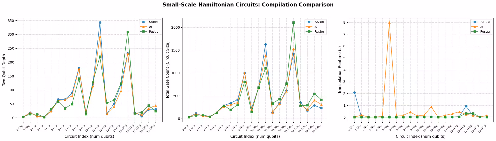
Графіки нижче порівнюють три методи за кожною метрикою для кожної схеми окремо. Схеми відсортовано за кількістю квітів і позначено за індексом на осі X, оскільки кілька схем можуть мати однакову кількість квітів.
def plot_transpilation_comparison(results, title_prefix):
    """
    Create a three-panel figure comparing compilation methods on
    two-qubit depth, circuit size, and runtime.

    Circuits are sorted by qubit count and plotted by circuit index.
    """
    methods = _method_order(results)
    palette = {"SABRE": "#1f77b4", "AI": "#ff7f0e", "Rustiq": "#2ca02c"}
    markers = {"SABRE": "o", "AI": "^", "Rustiq": "s"}

    # Order circuits by qubit count (then index) and map to plot positions
    ref = sorted(
        [r for r in results if r["method"] == methods[0]],
        key=lambda r: (r["num_qubits"], r["qc_index"]),
    )
    pos_map = {r["qc_index"]: pos for pos, r in enumerate(ref)}
    tick_positions = [pos_map[r["qc_index"]] for r in ref]
    tick_labels = [
        f"{pos_map[r['qc_index']]} ({r['num_qubits']}q)" for r in ref
    ]

    metrics = [
        ("two_qubit_depth", "Two-Qubit Depth"),
        ("size", "Total Gate Count (Circuit Size)"),
        ("runtime", "Transpilation Runtime (s)"),
    ]

    fig, axes = plt.subplots(1, 3, figsize=(20, 5.5))
    fig.suptitle(title_prefix, fontsize=15, fontweight="bold", y=1.02)

    for ax, (metric, ylabel) in zip(axes, metrics):
        for method in methods:
            subset = sorted(
                [r for r in results if r["method"] == method],
                key=lambda r: pos_map[r["qc_index"]],
            )
            ax.plot(
                [pos_map[r["qc_index"]] for r in subset],
                [r[metric] for r in subset],
                marker=markers.get(method, "o"),
                label=method,
                color=palette.get(method, None),
                linewidth=1.5,
                markersize=6,
                alpha=0.85,
            )
        ax.set_xlabel("Circuit Index (num qubits)", fontsize=11)
        ax.set_ylabel(ylabel, fontsize=11)
        ax.legend(frameon=True, fontsize=9)
        ax.grid(True, linestyle="--", alpha=0.4)
        step = max(1, len(tick_positions) // 15)
        ax.set_xticks(tick_positions[::step])
        ax.set_xticklabels(
            [tick_labels[i] for i in range(0, len(tick_labels), step)],
            fontsize=7,
            rotation=45,
            ha="right",
        )

    plt.tight_layout()
    plt.show()
def plot_pct_improvement_vs_sabre(results, title_prefix):
    """
    Plot the per-circuit percent improvement of each non-SABRE method
    relative to SABRE, for each metric. A positive value means the
    method improved on SABRE; negative means SABRE was better.
    """
    metrics = [
        ("two_qubit_depth", "2Q Depth"),
        ("size", "Gate Count"),
        ("runtime", "Runtime"),
    ]
    palette = {"AI": "#ff7f0e", "Rustiq": "#2ca02c"}
    markers = {"AI": "^", "Rustiq": "s"}

    methods = _method_order(results)
    sabre = sorted(
        [r for r in results if r["method"] == "SABRE"],
        key=lambda r: (r["num_qubits"], r["qc_index"]),
    )
    other_methods = [m for m in methods if m != "SABRE"]

    tick_positions = list(range(len(sabre)))
    tick_labels = [
        f"{i} ({sabre[i]['num_qubits']}q)" for i in range(len(sabre))
    ]

    fig, axes = plt.subplots(1, 3, figsize=(20, 5.5))
    fig.suptitle(
        f"{title_prefix}: % Improvement over SABRE",
        fontsize=15,
        fontweight="bold",
        y=1.02,
    )

    for ax, (metric, label) in zip(axes, metrics):
        ax.axhline(0, color="#1f77b4", linewidth=2, label="SABRE (baseline)")
        for method in other_methods:
            data = sorted(
                [r for r in results if r["method"] == method],
                key=lambda r: (r["num_qubits"], r["qc_index"]),
            )
            pct = [
                (sabre[i][metric] - data[i][metric]) / sabre[i][metric] * 100
                for i in range(len(sabre))
            ]
            ax.plot(
                tick_positions,
                pct,
                marker=markers.get(method, "o"),
                label=method,
                color=palette.get(method, None),
                linewidth=1.5,
                markersize=6,
                alpha=0.85,
            )
        ax.set_xlabel("Circuit Index (num qubits)", fontsize=11)
        ax.set_ylabel(f"% Improvement ({label})", fontsize=11)
        ax.legend(frameon=True, fontsize=9)
        ax.grid(True, linestyle="--", alpha=0.4)
        step = max(1, len(tick_positions) // 15)
        ax.set_xticks(tick_positions[::step])
        ax.set_xticklabels(
            [tick_labels[i] for i in range(0, len(tick_labels), step)],
            fontsize=7,
            rotation=45,
            ha="right",
        )
        ylims = ax.get_ylim()
        ax.axhspan(0, max(ylims[1], 1), alpha=0.04, color="green")
        ax.axhspan(min(ylims[0], -1), 0, alpha=0.04, color="red")

    plt.tight_layout()
    plt.show()
plot_transpilation_comparison(
    results_small,
    "Small-Scale Hamiltonian Circuits: Compilation Comparison",
)
plot_pct_improvement_vs_sabre(
    results_small,
    "Small-Scale Hamiltonian Circuits",
)
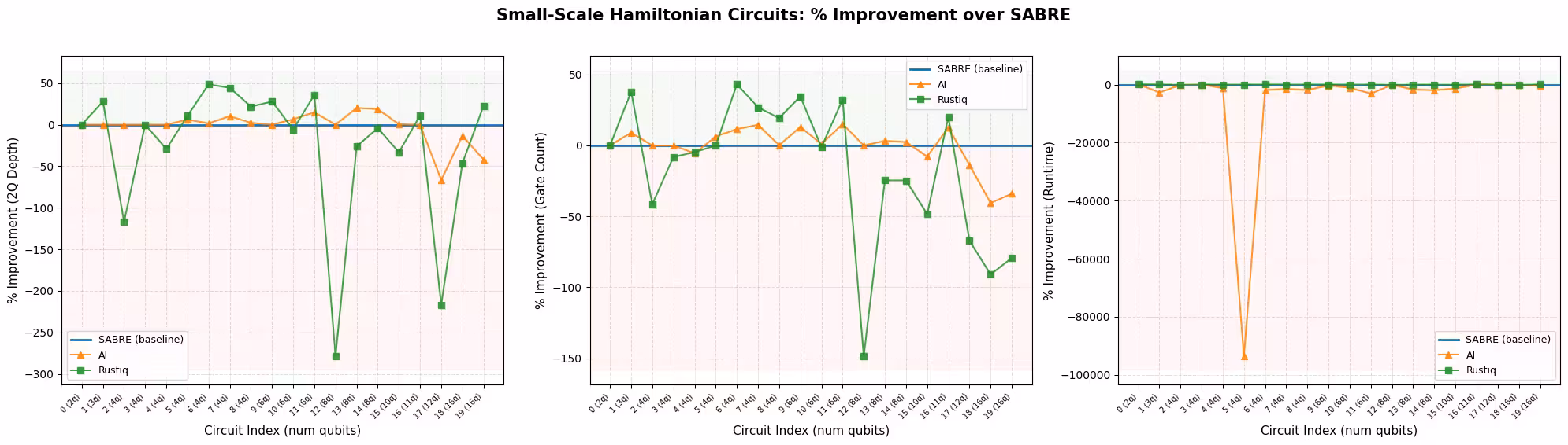
На цьому масштабі всі три менеджери проходів показують гарні результати, і їхні середні показники близькі один до одного. Це значною мірою пов'язано з тим, що малі схеми залишають обмежений простір для подальшої оптимізації, тому методи, як правило, сходяться до схожих рішень.
У цьому прикладі Rustiq дає найбільш змінні результати з найбільшими викидами як за двоквітною глибиною, так і за кількістю гейтів. Хоча ця мінливість означає, що іноді він відстає, вона також означає, що Rustiq іноді знаходить кращі рішення, ніж два інших методи. Транспілер AI демонструє більш стабільні результати відносно SABRE та Rustiq, дотримуючись близьких значень на більшості схем без суттєвих викидів.
За часом виконання SABRE та Rustiq обидва швидкі, тоді як транспілер з підтримкою AI помітно повільніший на певних схемах.
Найкращий метод за метрикою
Діаграма нижче показує, як часто кожен метод досягав найкращого (найнижчого) значення для кожної метрики. Нічиї можливі: для простіших схем кілька методів можуть досягти однакової оптимальної двоквітної глибини або кількості гейтів. Коли виникає нічия, усі зв'язані методи отримують залік, тому відсотки для конкретної метрики можуть перевищувати 100% у сумі.
def plot_best_method_bars(results, metrics_list=None):
    """
    Plot a grouped bar chart showing the percentage of circuits
    where each method achieved the best (lowest) value for each metric.

    Ties are counted for all tied methods, so percentages per metric
    can sum to more than 100%.
    """
    if metrics_list is None:
        metrics_list = ["two_qubit_depth", "size", "runtime"]

    labels = {
        "two_qubit_depth": "2Q Depth",
        "size": "Gate Count",
        "runtime": "Runtime",
    }
    methods = _method_order(results)
    palette = {"SABRE": "#1f77b4", "AI": "#ff7f0e", "Rustiq": "#2ca02c"}

    by_index = {}
    for r in results:
        by_index.setdefault(r["qc_index"], []).append(r)
    n_circuits = len(by_index)

    win_data = {m: [] for m in methods}
    tie_counts = []
    metric_labels = []

    for metric in metrics_list:
        metric_labels.append(
            labels.get(metric, metric.replace("_", " ").title())
        )
        counts = Counter()
        ties = 0
        for group in by_index.values():
            min_val = min(r[metric] for r in group)
            best = [r["method"] for r in group if r[metric] == min_val]
            if len(best) > 1:
                ties += 1
            counts.update(best)
        tie_counts.append(ties)
        for m in methods:
            win_data[m].append(counts.get(m, 0) / n_circuits * 100)

    x = np.arange(len(metric_labels))
    width = 0.22
    fig, ax = plt.subplots(figsize=(8, 5))

    for i, method in enumerate(methods):
        bars = ax.bar(
            x + i * width,
            win_data[method],
            width,
            label=method,
            color=palette.get(method, None),
            edgecolor="black",
            linewidth=0.5,
        )
        for bar in bars:
            height = bar.get_height()
            if height > 0:
                ax.text(
                    bar.get_x() + bar.get_width() / 2,
                    height + 1.5,
                    f"{height:.0f}%",
                    ha="center",
                    va="bottom",
                    fontsize=9,
                )

    # Annotate tie counts below each metric label
    for j, ties in enumerate(tie_counts):
        if ties > 0:
            ax.text(
                x[j] + width,
                -8,
                f"({ties} tie{'s' if ties != 1 else ''})",
                ha="center",
                va="top",
                fontsize=8,
                color="gray",
            )

    ax.set_xticks(x + width)
    ax.set_xticklabels(metric_labels, fontsize=11)
    ax.set_ylabel("Circuits with best value (%)", fontsize=11)
    ax.set_title(
        "Best-Performing Method by Metric (ties counted for all tied methods)",
        fontsize=12,
        fontweight="bold",
    )
    ax.legend(frameon=True, fontsize=10)
    ax.set_ylim(-12, 120)
    ax.yaxis.set_major_formatter(ticker.PercentFormatter())
    ax.grid(axis="y", linestyle="--", alpha=0.4)

    plt.tight_layout()
    plt.show()
plot_best_method_bars(results_small)

У цьому прикладі три методи працюють дуже схоже на малих схемах. За двоквітною глибиною та кількістю гейтів частка схем, у яких кожен метод є найкращим, близька (приблизно 35–55%), а багато схем закінчуються нічиєю, оскільки найпростіші схеми часто мають одне оптимальне рішення, яке знаходять кілька методів. Найчіткіша різниця стосується часу виконання: SABRE та Rustiq є найшвидшими приблизно на половині схем кожен, тоді як транспілер з підтримкою AI рідко буває найшвидшим. Беручи до уваги всі три метрики разом, Rustiq має незначну загальну перевагу він найчастіше перемагає за двоквітною глибиною і залишається конкурентоспроможним за кількістю гейтів та часом виконання.
Крок 3: Виконання за допомогою примітивів Qiskit
Щоб оцінити, як якість транспіляції впливає на виконання в умовах шуму, ми використовуємо техніку дзеркальних схем. Для кожної транспільованої схеми ми додаємо її обернену , щоб комбінована схема теоретично була тотожністю. Починаючи зі стану , ідеальне (безшумне) виконання повертало б рядок усіх нулів з імовірністю 1.
На практиці помилки гейтів накопичуються по всій схемі, тому ймовірність відновлення зменшується. Метод компіляції, який дає мілкішу схему з меншою кількістю гейтів, буде накопичувати менше шуму.
Підхід дзеркальних схем є привабливо простим і масштабується до будь-якого розміру схеми, оскільки очікуваний вихід завжди і класична симуляція ідеального стану не потрібна. Однак зверни увагу на такі застереження: дзеркальна схема є замінником реальної схеми (а не самою схемою), вона вдвічі збільшує кількість гейтів (що перебільшує ефект шуму), і вона може недооцінювати певні помилки, коли шум симетрично скасовується через межу дзеркала.
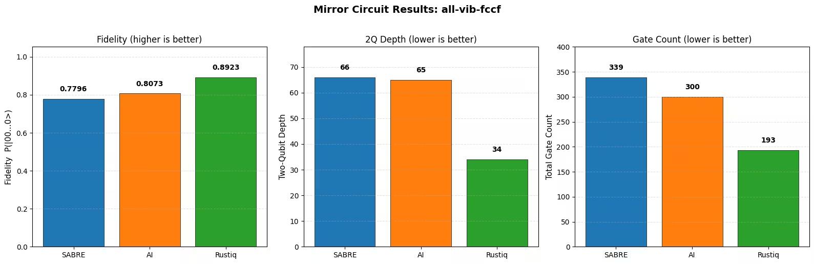
Ми обираємо схему з індексом 6 з малого набору та запускаємо дзеркальні схеми на симуляторі Aer з простою моделлю деполяризуючого шуму.
# Select circuit index 6 from the small-scale transpiled circuits
test_idx = 6
test_circuit = qc_small[test_idx]
print(f"Test circuit: {test_circuit.name}, {test_circuit.num_qubits} qubits")

# Get the transpiled versions
tqc_methods_small = {
    "SABRE": tqc_sabre_small[test_idx],
    "AI": tqc_ai_small[test_idx],
    "Rustiq": tqc_rustiq_small[test_idx],
}

# Show transpilation metrics for this circuit
print(f"\nTranspilation metrics for circuit index {test_idx}:")
for method, tqc in tqc_methods_small.items():
    depth_2q = tqc.depth(lambda x: x.operation.num_qubits == 2)
    size = tqc.size()
    print(f"  {method:8s}  2Q depth={depth_2q:5d}  size={size:6d}")
Test circuit: all-vib-fccf, 4 qubits

Transpilation metrics for circuit index 6:
  SABRE     2Q depth=   66  size=   339
  AI        2Q depth=   65  size=   300
  Rustiq    2Q depth=   34  size=   193
Побудуй дзеркальні схеми (додай ), перемапуй на суміжні індекси квітів, щоб симулятор обробляв лише активні квіти, і запусти на шумному симуляторі Aer.
def remap_to_contiguous(tqc):
    """Remap a transpiled circuit to use contiguous qubit indices.

    Transpiled circuits target specific physical qubits (e.g., qubit 45, 67)
    on a large backend. This remaps them to 0, 1, 2, ... so Aer only
    simulates the active qubits.
    """
    active = sorted(
        {tqc.find_bit(q).index for inst in tqc.data for q in inst.qubits}
    )
    qubit_map = {old: new for new, old in enumerate(active)}
    new_qc = QuantumCircuit(len(active))
    for inst in tqc.data:
        old_indices = [tqc.find_bit(q).index for q in inst.qubits]
        new_qc.append(inst.operation, [qubit_map[i] for i in old_indices])
    return new_qc

def build_mirror_circuit(tqc):
    """Build a mirror circuit: U followed by U-dagger, with measurements.

    The combined circuit U-dagger @ U should be the identity, so measuring
    all zeros indicates a noise-free execution.
    """
    tqc_compact = remap_to_contiguous(tqc)
    mirror = tqc_compact.compose(tqc_compact.inverse())
    mirror.measure_all()
    return mirror

# Build a simple depolarizing noise model
noise_model = NoiseModel()
noise_model.add_all_qubit_quantum_error(
    depolarizing_error(0.001, 1),
    ["sx", "x", "rz"],  # ~0.1% per 1Q gate
)
noise_model.add_all_qubit_quantum_error(
    depolarizing_error(0.01, 2),
    ["cx", "ecr"],  # ~1% per 2Q gate
)

aer_sim = AerSimulator(noise_model=noise_model)

shots = 10000
fidelities = {}

for method, tqc in tqc_methods_small.items():
    mirror = build_mirror_circuit(tqc)

    sampler = SamplerV2(mode=aer_sim)
    job = sampler.run([mirror], shots=shots)
    result = job.result()
    counts = result[0].data.meas.get_counts()

    # Fidelity = fraction of all-zeros (error-free) outcomes
    n_qubits = mirror.num_qubits - mirror.num_clbits  # active qubits
    all_zeros = "0" * mirror.num_qubits
    fidelity = counts.get(all_zeros, 0) / shots
    fidelities[method] = fidelity
    print(
        f"{method:8s}  P(|00...0>) = {fidelity:.4f}  ({counts.get(all_zeros, 0)}/{shots})"
    )
SABRE     P(|00...0>) = 0.7796  (7796/10000)
AI        P(|00...0>) = 0.8073  (8073/10000)
Rustiq    P(|00...0>) = 0.8923  (8923/10000)
def plot_mirror_results(tqc_methods, fidelities, circuit_name):
    """
    Plot a three-panel comparison: fidelity, 2Q depth,
    and gate count for each compilation method.
    """
    methods = list(tqc_methods.keys())
    palette = {"SABRE": "#1f77b4", "AI": "#ff7f0e", "Rustiq": "#2ca02c"}
    colors = [palette.get(m, "gray") for m in methods]

    fidelity_vals = [fidelities[m] for m in methods]
    depth_vals = [
        tqc_methods[m].depth(lambda x: x.operation.num_qubits == 2)
        for m in methods
    ]
    size_vals = [tqc_methods[m].size() for m in methods]

    fig, axes = plt.subplots(1, 3, figsize=(16, 5))
    fig.suptitle(
        f"Mirror Circuit Results: {circuit_name}",
        fontsize=14,
        fontweight="bold",
        y=1.02,
    )

    def _annotate_bars(ax, bars, values, fmt="{}"):
        ymax = ax.get_ylim()[1]
        for bar, val in zip(bars, values):
            label = fmt.format(val)
            y = val + ymax * 0.03
            ax.text(
                bar.get_x() + bar.get_width() / 2,
                y,
                label,
                ha="center",
                va="bottom",
                fontsize=10,
                fontweight="bold",
            )

    # Panel 1: Survival Probability
    bars = axes[0].bar(
        methods, fidelity_vals, color=colors, edgecolor="black", linewidth=0.5
    )
    axes[0].set_ylabel("Fidelity  P(|00...0>)", fontsize=11)
    axes[0].set_title("Fidelity (higher is better)", fontsize=12)
    axes[0].set_ylim(
        0, max(fidelity_vals) * 1.18 if max(fidelity_vals) > 0 else 1.0
    )
    axes[0].grid(axis="y", linestyle="--", alpha=0.4)
    _annotate_bars(axes[0], bars, fidelity_vals, fmt="{:.4f}")

    # Panel 2: Two-Qubit Depth
    bars = axes[1].bar(
        methods, depth_vals, color=colors, edgecolor="black", linewidth=0.5
    )
    axes[1].set_ylabel("Two-Qubit Depth", fontsize=11)
    axes[1].set_title("2Q Depth (lower is better)", fontsize=12)
    axes[1].set_ylim(0, max(depth_vals) * 1.18)
    axes[1].grid(axis="y", linestyle="--", alpha=0.4)
    _annotate_bars(axes[1], bars, depth_vals)

    # Panel 3: Gate Count
    bars = axes[2].bar(
        methods, size_vals, color=colors, edgecolor="black", linewidth=0.5
    )
    axes[2].set_ylabel("Total Gate Count", fontsize=11)
    axes[2].set_title("Gate Count (lower is better)", fontsize=12)
    axes[2].set_ylim(0, max(size_vals) * 1.18)
    axes[2].grid(axis="y", linestyle="--", alpha=0.4)
    _annotate_bars(axes[2], bars, size_vals)

    plt.tight_layout()
    plt.show()

plot_mirror_results(tqc_methods_small, fidelities, test_circuit.name)
Спостереження
Метод з найменшою двоквітною глибиною та найменшою кількістю гейтів досягає найвищої точності, що відповідає очікуванню про те, що коротші схеми накопичують менше шуму. Навіть невеликі відмінності в глибині та кількості гейтів призводять до відчутних відмінностей у точності при деполяризуючій моделі шуму.
Пам'ятай, що ці результати стосуються однієї схеми. Відносне ранжування методів може змінюватись від схеми до схеми залежно від структури гамільтоніана.
Приклад великого масштабу на реальному апаратному забезпеченні
У цьому розділі ми порівнюємо ті самі три методи компіляції на схемах гамільтоніана з 20 або більше квітами. Ці схеми більш репрезентативні для практичних задач симуляції гамільтоніана та дозволяють перевірити, як кожен метод масштабується з точки зору якості схеми та часу компіляції.
Кроки 1–4 разом
Робочий процес відповідає тій самій структурі, що й приклад малого масштабу. Ми транспілюємо всі великі схеми кожним методом, збираємо метрики та надсилаємо дзеркальну схему на реальне квантове апаратне забезпечення.
results_large = []

tqc_sabre_large = capture_transpilation_metrics(
    results_large, pm_sabre, qc_large, "SABRE"
)
tqc_ai_large = capture_transpilation_metrics(
    results_large, pm_ai, qc_large, "AI"
)
tqc_rustiq_large = capture_transpilation_metrics(
    results_large, pm_rustiq, qc_large, "Rustiq"
)
[SABRE] Circuit 0 (all-vib-hc3h2cn): 2Q depth=2, size=258, time=0.16s
[SABRE] Circuit 1 (ham-graph-gnp_k-5): 2Q depth=345, size=4036, time=0.08s
[SABRE] Circuit 2 (TSP_Ncity-5): 2Q depth=187, size=2045, time=0.04s
[SABRE] Circuit 3 (tfim): 2Q depth=100, size=489, time=0.21s
[SABRE] Circuit 4 (all-vib-h2co): 2Q depth=30, size=570, time=0.18s
[SABRE] Circuit 5 (uuf100-ham): 2Q depth=414, size=4779, time=0.09s
[SABRE] Circuit 6 (uuf100-ham): 2Q depth=523, size=5667, time=0.11s
[SABRE] Circuit 7 (graph-gnp_k-4): 2Q depth=3028, size=24885, time=0.39s
[SABRE] Circuit 8 (uf100-ham): 2Q depth=700, size=8271, time=0.15s
[SABRE] Circuit 9 (uf100-ham): 2Q depth=698, size=8957, time=0.15s
[SABRE] Circuit 10 (TSP_Ncity-7): 2Q depth=432, size=6353, time=0.12s
[SABRE] Circuit 11 (all-vib-cyclo_propene): 2Q depth=30, size=1144, time=0.20s
[SABRE] Circuit 12 (TSP_Ncity-8): 2Q depth=704, size=10287, time=0.18s
[SABRE] Circuit 13 (uf100-ham): 2Q depth=2454, size=30195, time=0.46s
[SABRE] Circuit 14 (tfim): 2Q depth=245, size=3670, time=0.08s
[SABRE] Circuit 15 (flat100-ham): 2Q depth=154, size=3836, time=0.12s
[SABRE] Circuit 16 (graph-regular_reg-4): 2Q depth=863, size=14063, time=0.22s
[SABRE] Circuit 17 (tfim): 2Q depth=581, size=8810, time=0.15s
[SABRE] Circuit 18 (FH_D-1): 2Q depth=1704, size=9528, time=0.35s
[SABRE] Circuit 19 (TSP_Ncity-10): 2Q depth=1091, size=22041, time=0.38s
[SABRE] Circuit 20 (TSP_Ncity-10): 2Q depth=1091, size=22005, time=0.38s
[SABRE] Circuit 21 (ham-unary-color02-queen13_13_k-4): 2Q depth=224, size=8321, time=0.17s
[AI] Circuit 0 (all-vib-hc3h2cn): 2Q depth=2, size=258, time=0.17s
[AI] Circuit 1 (ham-graph-gnp_k-5): 2Q depth=323, size=4418, time=3.13s
[AI] Circuit 2 (TSP_Ncity-5): 2Q depth=161, size=2229, time=1.47s
[AI] Circuit 3 (tfim): 2Q depth=20, size=402, time=0.34s
[AI] Circuit 4 (all-vib-h2co): 2Q depth=38, size=661, time=0.19s
[AI] Circuit 5 (uuf100-ham): 2Q depth=391, size=5130, time=3.27s
[AI] Circuit 6 (uuf100-ham): 2Q depth=463, size=6095, time=4.23s
[AI] Circuit 7 (graph-gnp_k-4): 2Q depth=3207, size=25641, time=15.15s
[AI] Circuit 8 (uf100-ham): 2Q depth=637, size=8267, time=5.87s
[AI] Circuit 9 (uf100-ham): 2Q depth=632, size=9330, time=7.29s
[AI] Circuit 10 (TSP_Ncity-7): 2Q depth=452, size=7418, time=6.02s
[AI] Circuit 11 (all-vib-cyclo_propene): 2Q depth=38, size=1323, time=0.27s
[AI] Circuit 12 (TSP_Ncity-8): 2Q depth=609, size=11131, time=10.07s
[AI] Circuit 13 (uf100-ham): 2Q depth=2251, size=31128, time=38.77s
[AI] Circuit 14 (tfim): 2Q depth=165, size=3460, time=1.64s
[AI] Circuit 15 (flat100-ham): 2Q depth=91, size=3497, time=2.49s
[AI] Circuit 16 (graph-regular_reg-4): 2Q depth=664, size=15256, time=12.35s
[AI] Circuit 17 (tfim): 2Q depth=583, size=9157, time=6.28s
[AI] Circuit 18 (FH_D-1): 2Q depth=1193, size=7754, time=4.54s
[AI] Circuit 19 (TSP_Ncity-10): 2Q depth=1134, size=22577, time=25.64s
[AI] Circuit 20 (TSP_Ncity-10): 2Q depth=1172, size=23851, time=28.97s
[AI] Circuit 21 (ham-unary-color02-queen13_13_k-4): 2Q depth=219, size=8600, time=8.85s
[Rustiq] Circuit 0 (all-vib-hc3h2cn): 2Q depth=2, size=257, time=0.16s
[Rustiq] Circuit 1 (ham-graph-gnp_k-5): 2Q depth=640, size=5831, time=0.13s
[Rustiq] Circuit 2 (TSP_Ncity-5): 2Q depth=408, size=3985, time=0.08s
[Rustiq] Circuit 3 (tfim): 2Q depth=31, size=688, time=0.07s
[Rustiq] Circuit 4 (all-vib-h2co): 2Q depth=65, size=1058, time=2.91s
[Rustiq] Circuit 5 (uuf100-ham): 2Q depth=633, size=6757, time=0.14s
[Rustiq] Circuit 6 (uuf100-ham): 2Q depth=795, size=8495, time=0.17s
[Rustiq] Circuit 7 (graph-gnp_k-4): 2Q depth=13768, size=139793, time=2.92s
[Rustiq] Circuit 8 (uf100-ham): 2Q depth=1099, size=11878, time=0.25s
[Rustiq] Circuit 9 (uf100-ham): 2Q depth=911, size=11111, time=0.22s
[Rustiq] Circuit 10 (TSP_Ncity-7): 2Q depth=1183, size=13197, time=0.27s
[Rustiq] Circuit 11 (all-vib-cyclo_propene): 2Q depth=67, size=2491, time=13.56s
[Rustiq] Circuit 12 (TSP_Ncity-8): 2Q depth=1615, size=21358, time=0.48s
[Rustiq] Circuit 13 (uf100-ham): 2Q depth=2920, size=40465, time=0.91s
[Rustiq] Circuit 14 (tfim): 2Q depth=489, size=6552, time=0.15s
[Rustiq] Circuit 15 (flat100-ham): 2Q depth=378, size=5906, time=0.14s
[Rustiq] Circuit 16 (graph-regular_reg-4): 2Q depth=12163, size=168679, time=2.94s
[Rustiq] Circuit 17 (tfim): 2Q depth=1208, size=17042, time=0.36s
[Rustiq] Circuit 18 (FH_D-1): 2Q depth=1061, size=24000, time=0.47s
[Rustiq] Circuit 19 (TSP_Ncity-10): 2Q depth=2565, size=41340, time=1.38s
[Rustiq] Circuit 20 (TSP_Ncity-10): 2Q depth=2565, size=41275, time=1.38s
[Rustiq] Circuit 21 (ham-unary-color02-queen13_13_k-4): 2Q depth=808, size=17548, time=0.42s
print_summary_table(results_large)
Mean +/- std per compilation method
Method                2Q Depth              Gate Count             Runtime (s)
------------------------------------------------------------------------------
SABRE          709.1 +/- 783.8     9,100.5 +/- 8,493.1             0.2 +/- 0.1
AI             656.6 +/- 777.5     9,435.6 +/- 8,853.0            8.5 +/- 10.2
Rustiq     2,062.5 +/- 3,631.1   26,804.8 +/- 43,403.1             1.3 +/- 2.9

Mean % improvement vs SABRE (positive = better than SABRE)
Method                2Q Depth              Gate Count             Runtime (s)
------------------------------------------------------------------------------
AI             +9.6% +/- 22.8%          -3.4% +/- 9.4%    -3620.0% +/- 2405.5%
Rustiq      -154.5% +/- 273.9%      -137.1% +/- 233.2%     -527.0% +/- 1405.5%
print_per_circuit_comparison(results_large, num_rows=8)
2Q Depth (first 8 circuits by qubit count); * = best
Idx  Circuit            Q    SABRE       AI   Rustiq
----------------------------------------------------
  0  all-vib-hc3h2cn   24       2*       2*       2*
  1  ham-graph-gnp_k-  24      345     323*      640
  2  TSP_Ncity-5       25      187     161*      408
  3  tfim              26      100      20*       31
  4  all-vib-h2co      32      30*       38       65
  5  uuf100-ham        40      414     391*      633
  6  uuf100-ham        40      523     463*      795
  7  graph-gnp_k-4     40    3028*     3207    13768

Gate Count (first 8 circuits by qubit count); * = best
Idx  Circuit            Q    SABRE       AI   Rustiq
----------------------------------------------------
  0  all-vib-hc3h2cn   24      258      258     257*
  1  ham-graph-gnp_k-  24    4036*     4418     5831
  2  TSP_Ncity-5       25    2045*     2229     3985
  3  tfim              26      489     402*      688
  4  all-vib-h2co      32     570*      661     1058
  5  uuf100-ham        40    4779*     5130     6757
  6  uuf100-ham        40    5667*     6095     8495
  7  graph-gnp_k-4     40   24885*    25641   139793

Runtime (s) (first 8 circuits by qubit count); * = best
Idx  Circuit            Q    SABRE       AI   Rustiq
----------------------------------------------------
  0  all-vib-hc3h2cn   24     0.16     0.17    0.16*
  1  ham-graph-gnp_k-  24    0.08*     3.13     0.13
  2  TSP_Ncity-5       25    0.04*     1.47     0.08
  3  tfim              26     0.21     0.34    0.07*
  4  all-vib-h2co      32    0.18*     0.19     2.91
  5  uuf100-ham        40    0.09*     3.27     0.14
  6  uuf100-ham        40    0.11*     4.23     0.17
  7  graph-gnp_k-4     40    0.39*    15.15     2.92
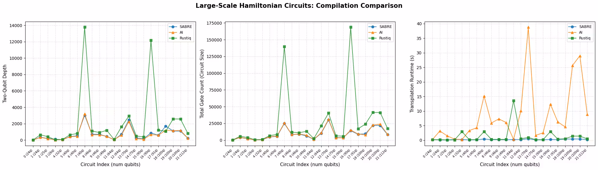
plot_transpilation_comparison(
    results_large,
    "Large-Scale Hamiltonian Circuits: Compilation Comparison",
)
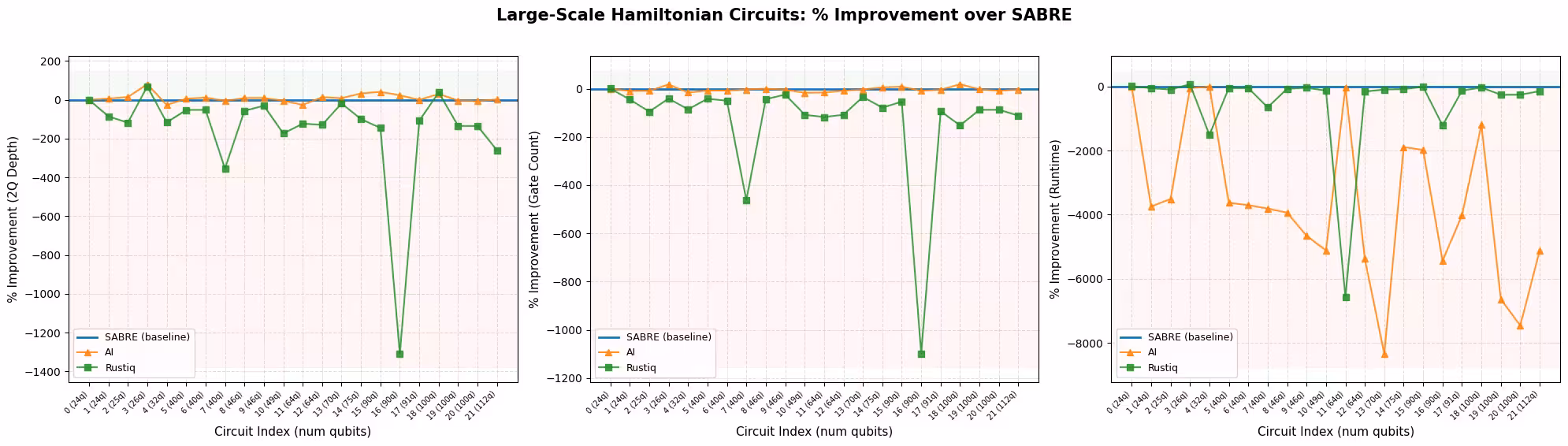
plot_pct_improvement_vs_sabre(
    results_large,
    "Large-Scale Hamiltonian Circuits",
)
plot_best_method_bars(results_large)

# Select circuit index 3 from the large-scale transpiled circuits
test_idx_large = 3
test_circuit_large = qc_large[test_idx_large]
print(
    f"Test circuit: {test_circuit_large.name}, {test_circuit_large.num_qubits} qubits"
)

tqc_methods_large = {
    "SABRE": tqc_sabre_large[test_idx_large],
    "AI": tqc_ai_large[test_idx_large],
    "Rustiq": tqc_rustiq_large[test_idx_large],
}

print(f"\nTranspilation metrics for circuit index {test_idx_large}:")
for method, tqc in tqc_methods_large.items():
    depth_2q = tqc.depth(lambda x: x.operation.num_qubits == 2)
    size = tqc.size()
    print(f"  {method:8s}  2Q depth={depth_2q:5d}  size={size:6d}")
Test circuit: tfim, 26 qubits

Transpilation metrics for circuit index 3:
  SABRE     2Q depth=  100  size=   489
  AI        2Q depth=   20  size=   402
  Rustiq    2Q depth=   31  size=   688
pm_mirror = generate_preset_pass_manager(
    optimization_level=0, backend=backend
)

for method, tqc in tqc_methods_large.items():
    # print the count ops for each circuit
    mirror = tqc.copy()
    mirror.compose(tqc.inverse(), inplace=True)
    mirror.measure_all()
    mirror = pm_mirror.run(mirror)
    print(f"\n{method} transpiled circuit:")
    print(tqc.count_ops())
    print(f"{method} mirror circuit count ops:")
    print(mirror.count_ops())
SABRE transpiled circuit:
OrderedDict({'sx': 211, 'rz': 163, 'cz': 104, 'x': 11})
SABRE mirror circuit count ops:
OrderedDict({'rz': 1170, 'sx': 422, 'cz': 208, 'measure': 156, 'x': 22, 'barrier': 1})

AI transpiled circuit:
OrderedDict({'sx': 165, 'rz': 162, 'cz': 68, 'x': 7})
AI mirror circuit count ops:
OrderedDict({'rz': 984, 'sx': 330, 'measure': 156, 'cz': 136, 'x': 14, 'barrier': 1})

Rustiq transpiled circuit:
OrderedDict({'sx': 316, 'rz': 225, 'cz': 140, 'x': 7})
Rustiq mirror circuit count ops:
OrderedDict({'rz': 1714, 'sx': 632, 'cz': 280, 'measure': 156, 'x': 14, 'barrier': 1})
# Build mirror circuits and submit to real hardware
# The inverse may introduce gates (e.g., sxdg) not in the backend's
# basis gate set, so we re-transpile the mirror circuit.
pm_mirror = generate_preset_pass_manager(
    optimization_level=0, backend=backend
)

shots_hw = 10000
hw_jobs = {}

for method, tqc in tqc_methods_large.items():
    mirror = tqc.copy()
    mirror.compose(tqc.inverse(), inplace=True)
    mirror.measure_all()

    # Re-transpile at opt level 0 to decompose into basis gates
    # without changing the layout or routing
    mirror = pm_mirror.run(mirror)

    sampler = SamplerV2(mode=backend)
    sampler.options.environment.job_tags = ["TUT_CMHSC"]
    job = sampler.run([mirror], shots=shots_hw)
    hw_jobs[method] = job
    print(f"{method}: submitted job {job.job_id()}")
SABRE: submitted job d8gvgq66983c73dqe5og
AI: submitted job d8gvgqe6983c73dqe5pg
Rustiq: submitted job d8gvgqm6983c73dqe5q0
# Retrieve results and compute fidelities
fidelities_large = {}

for method, job in hw_jobs.items():
    result = job.result()
    counts = result[0].data.meas.get_counts()

    n_qubits = backend.num_qubits
    all_zeros = "0" * n_qubits
    fidelity = counts.get(all_zeros, 0) / shots_hw
    fidelities_large[method] = fidelity
    print(
        f"{method:8s}  P(|00...0>) = {fidelity:.4f}  ({counts.get(all_zeros, 0)}/{shots_hw})"
    )
SABRE     P(|00...0>) = 0.0005  (5/10000)
AI        P(|00...0>) = 0.3267  (3267/10000)
Rustiq    P(|00...0>) = 0.1845  (1845/10000)
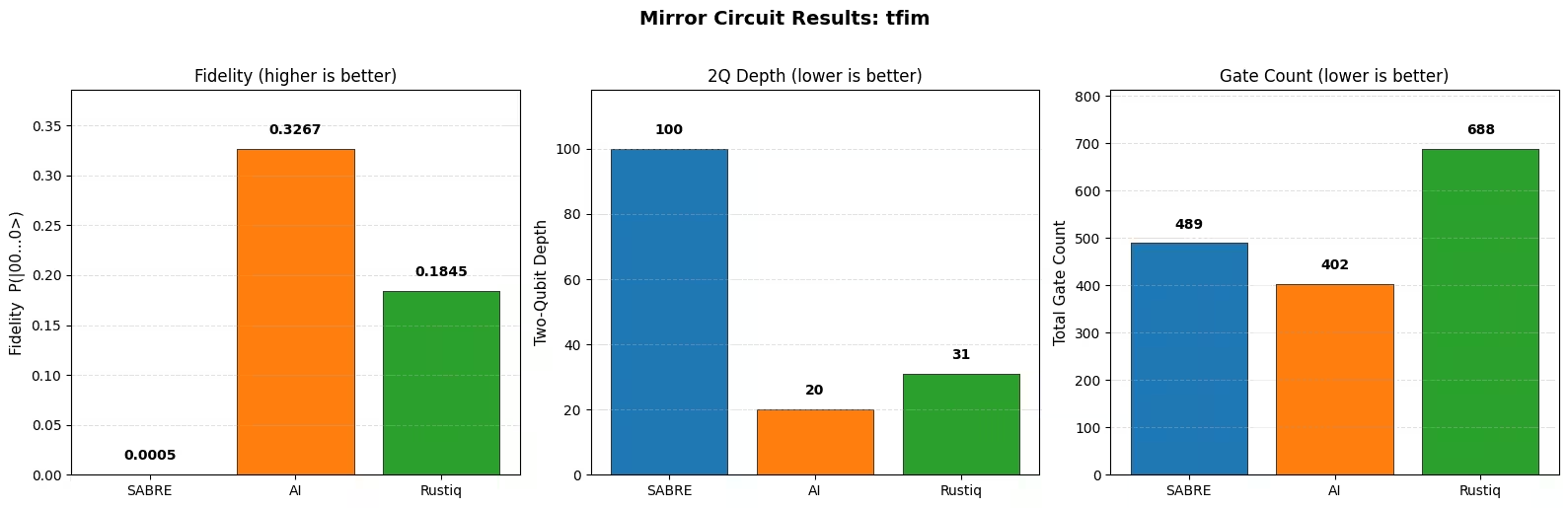
plot_mirror_results(
    tqc_methods_large, fidelities_large, test_circuit_large.name
)
Аналіз результатів компіляції
Бенчмарки вище порівнюють SABRE, транспілер з підтримкою AI та Rustiq на схемах симуляції гамільтоніана з колекції Hamlib як у малому, так і у великому масштабі.
Двоквітна глибина та кількість гейтів
На великому масштабі SABRE та транспілер з підтримкою AI є двома найкращими виконавцями, і кожен лідирує за різною метрикою. Як показує діаграма найкращого методу за метрикою, SABRE виробляє найменшу кількість гейтів для переважної більшості схем і є найшвидшим методом майже на всіх схемах, що відповідає евристиці, розробленій для мінімізації вставлених гейтів SWAP, і нещодавнім оптимізаціям компонування та маршрутизації. Транспілер з підтримкою AI виробляє найменшу двоквітну глибину на більшості схем, що відповідає частині його мети навчання з підкріпленням, яка спрямована на глибину схеми. Зведена таблиця відображає той самий поділ: SABRE має меншу середню кількість гейтів, тоді як транспілер AI має меншу середню двоквітну глибину. Обидва методи є послідовними та надійними для всього діапазону схем.
Rustiq, спеціально створений для синтезу PauliEvolutionGate, виробляє єдиний найкращий результат лише для невеликої частки великомасштабних схем. Його середні метрики сильно спотворені кількома значними викидами, помітними як великі піки на графіку порівняння компіляції, де Rustiq виробляє суттєво більшу глибину та кількість гейтів, ніж інші методи. Без цих викидів його середня продуктивність була б набагато ближчою до SABRE та транспілера з підтримкою AI.
Ключове спостереження полягає в тому, що жоден окремий метод не домінує на кожній схемі. Кожен метод перевершує інші в конкретних випадках, що робить доцільним спробувати всі доступні інструменти та вибрати найкращий результат для кожної схеми.
Час виконання
SABRE послідовно є найшвидшим методом. Rustiq зазвичай працює з подібною швидкістю, але може виробляти викиди, де компіляція займає значно більше часу. Це особливо помітно у великих результатах, де кілька схем змушують час виконання Rustiq стрімко зростати. Ці викиди суттєво впливають на середній час виконання, тому медіана може бути більш репрезентативним підсумком для Rustiq. Транспілер з підтримкою AI є найповільнішим із трьох, з часом виконання, який помітно зростає на більших і складніших схемах.
Результати дзеркальних схем
Експерименти з дзеркальними схемами підтверджують очікувану тенденцію: методи, що виробляють меншу двоквітну глибину та меншу кількість гейтів, досягають вищої точності в умовах шуму. Це виконується як на шумному симуляторі (малий масштаб), так і на реальному апаратному забезпеченні (великий масштаб).
Пам'ятай, що кожен графік дзеркальної схеми відображає одну схему, а не загальне. Приклад апаратного забезпечення вище використовує одну схему tfim на 26 квітах, яка в даному випадку є прикладом, де SABRE виробляє значно більшу двоквітну глибину, ніж транспілер з підтримкою AI та Rustiq, тому його точність відповідно набагато нижча. Це не є репрезентативним для ширших результатів: у повному наборі великомасштабних схем двоквітна глибина SABRE зазвичай близька до двоквітної глибини транспілера з підтримкою AI, і обидва методи лідирують за різними метриками (транспілер з підтримкою AI за двоквітною глибиною, SABRE за кількістю гейтів та часом виконання). Один результат дзеркальної схеми тестує подвоєну версію однієї схеми, а не повне навантаження, тому його не слід сприймати як вирок щодо загальної якості методу.
Рекомендації
Не існує єдиної найкращої стратегії транспіляції для всіх схем. Найкращий вибір залежить від структури схеми, мети оптимізації та доступного бюджету часу компіляції:
- SABRE є рекомендованим стандартним вибором. Він швидкий і надійний, та виробляє сильні результати для широкого діапазону схем. Для подальшого налаштування користувачі можуть збільшити кількість спроб компонування та маршрутизації (дивись підручник з оптимізації SABRE).
- Транспілер з підтримкою AI варто спробувати, коли час компіляції не є обмеженням, особливо коли пріоритетом є мінімізація двоквітної глибини: він виробив найменшу двоквітну глибину на більшості великомасштабних схем у цьому бенчмарку.
- Rustiq спеціально створений для схем
PauliEvolutionGateі може знаходити рішення з дуже малою глибиною та невеликою кількістю гейтів, особливо на менших схемах. На більших схемах він іноді може виробляти значно більші результати, тому його найкраще використовувати як один із кількох методів для спроби, а не як стандартний вибір.
На практиці найкращий підхід — запустити всі доступні методи та вибрати найкращий результат для кожної схеми. Накладні витрати компіляції від спроби кількох методів невеликі порівняно з потенційним покращенням якості виконання на реальному апаратному забезпеченні.
Наступні кроки
Якщо цей підручник виявився корисним, тебе можуть зацікавити такі матеріали:
Посилання
[1] "LightSABRE: A Lightweight and Enhanced SABRE Algorithm". H. Zou, M. Treinish, K. Hartman, A. Ivrii, J. Lishman et al. https://arxiv.org/abs/2409.08368
[2] "Practical and efficient quantum circuit synthesis and transpiling with Reinforcement Learning". D. Kremer, V. Villar, H. Paik, I. Duran, I. Faro, J. Cruz-Benito et al. https://arxiv.org/abs/2405.13196
[3] "Pauli Network Circuit Synthesis with Reinforcement Learning". A. Dubal, D. Kremer, S. Martiel, V. Villar, D. Wang, J. Cruz-Benito et al. https://arxiv.org/abs/2503.14448
[4] "Faster and shorter synthesis of Hamiltonian simulation circuits". T. Goubault de Brugiere, S. Martiel et al. https://arxiv.org/abs/2404.03280