Розігрів QAOA (warm-start) за допомогою аддону Qiskit Optimization Mapper

Орієнтовний час використання: 9 хвилин на Heron r3 (ПРИМІТКА: це лише орієнтовна оцінка. Твій фактичний час може відрізнятися.)

Результати навчання

• Як відобразити задачу max-cut на квантову формулювання квадратичної безумовної бінарної оптимізації (QUBO) за допомогою qiskit-addon-opt-mapper

• Як реалізувати та запустити стандартний QAOA на симуляторі

• Як застосувати WS-QAOA, обчисливши релаксацію квадратичної програми (QP) і побудувавши схему з розігрівом (warm-start)

• Як порівняти збіжність енергії та якість розв'язку між стандартним QAOA та WS-QAOA

Передумови

• Навчальний посібник із QAOA

• Розширений навчальний посібник із QAOA

Передумови

Квантовий алгоритм наближеної оптимізації (QAOA) — це гібридний квантово-класичний алгоритм, розроблений для розв'язання задач комбінаторної оптимізації, таких як max-cut і загальні формулювання QUBO. Базовий вступ до QAOA у Qiskit див. у навчальному посібнику з QAOA; складніші техніки побудови схем описано в розширеному навчальному посібнику з QAOA.

У стандартному QAOA:

• Початковим станом є однорідна суперпозиція $|+\rangle^{\otimes n}$.
• Варіаційні параметри ініціалізуються випадково.
• Класичний оптимізатор шукає параметри, що мінімізують функцію вартості.

Однак для практичних розмірів задач і зашумленого квантового апаратного забезпечення випадкова ініціалізація може призвести до повільної збіжності, поганих локальних мінімумів і збільшення вартості оптимізації.

Розігрів QAOA (WS-QAOA) покращує це, безпосередньо вбудовуючи класичні оптимізаційні знання у квантову схему. Цей навчальний посібник дотримується методів, представлених Egger, Mareček і Woerner у статті Warm-starting quantum optimization. Ключова ідея полягає в тому, щоб:

1. Розв'язати неперервну релаксацію початкової бінарної задачі (квадратичну програму над $[0,1]^n$ замість $\{0,1\}^n$).

2. Закодувати релаксований розв'язок $c^*_i \in [0,1]$ у власний початковий стан за допомогою кутів $Y$-обертання $\theta_i = 2\arcsin(\sqrt{c^*_i})$, так щоб кубіт $i$ починав у стані, ймовірність вимірювання якого як $|1\rangle$ дорівнює $c^*_i$.

3. Замінити стандартний $X$-мікшер власним мікшером, основний стан якого є початковим станом розігріву, гарантуючи, що алгоритм починає роботу поблизу класичного розв'язку і може досліджувати його околиці.

Параметр регуляризації $\varepsilon \in [0, 0.5]$ обрізає $c^*_i$ від 0 і 1, щоб уникнути проблем із досяжністю; кубіти, ініціалізовані у стані $|0\rangle$ або $|1\rangle$, не можуть бути переміщені гамільтоніаном вартості. При $\varepsilon = 0.5$ WS-QAOA точно зводиться до стандартного QAOA.

Моделювання задачі використовує пакет qiskit-addon-opt-mapper, клас застосунку якого Maxcut будує QUBO безпосередньо з графа, а конвертери та транслятори відображають отриману задачу на квантові гамільтоніани.

Вимоги

Перш ніж почати цей навчальний посібник, переконайся, що встановлено таке:

• Qiskit SDK версії 2.0 або новішої, з підтримкою візуалізації

• Qiskit Runtime версії 0.43 або новішої (pip install qiskit-ibm-runtime)

• Аддон Qiskit Optimization Mapper (pip install qiskit-addon-opt-mapper)

• SciPy (pip install scipy)

• NetworkX (pip install networkx)

Налаштування

Імпортуй усі необхідні бібліотеки та визнач допоміжні функції, що використовуються протягом цього навчального посібника.

# Added by doQumentation — required packages for this notebook
!pip install -q matplotlib networkx numpy qiskit qiskit-addon-opt-mapper qiskit-ibm-runtime scipy

import numpy as np
import matplotlib.pyplot as plt
import networkx as nx
from scipy.optimize import minimize

from qiskit.circuit import QuantumCircuit, ParameterVector
from qiskit.circuit.library import qaoa_ansatz
from qiskit.quantum_info import Statevector
from qiskit.primitives import StatevectorEstimator, StatevectorSampler
from qiskit.transpiler.preset_passmanagers import generate_preset_pass_manager
from qiskit_ibm_runtime import (
    QiskitRuntimeService,
    Session,
    EstimatorOptions,
    EstimatorV2 as Estimator,
    SamplerV2 as Sampler,
)

from qiskit_addon_opt_mapper.applications import Maxcut
from qiskit_addon_opt_mapper.converters import OptimizationProblemToQubo
from qiskit_addon_opt_mapper.translators import to_ising

Приклад малого симулятора

Як наскрізний приклад ми використовуємо невелику задачу max-cut на зваженому графі. Max-cut запитує: маючи граф $G=(V,E)$ з вагами ребер $w_{ij}$, знайти розбиття вершин на дві множини $S$ і $\bar{S}$, що максимізує сумарну вагу ребер, які перетинають розріз.

Як задачу мінімізації QUBO max-cut можна записати так: $\min_{x \in \{0,1\}^n} -\sum_{(i,j) \in E} w_{ij}(x_i + x_j - 2x_i x_j)$

Ми працюємо з графом із чотирма вузлами, щоб зберегти прийнятність обчислень на симуляторі.

Крок 1: відобразити класичні вхідні дані на квантову задачу

Ми визначаємо задачу max-cut за допомогою класу застосунку Maxcut з qiskit-addon-opt-mapper, який будує формулювання QUBO безпосередньо з графа. Потім ми перетворюємо її на QUBO і транслюємо в гамільтоніан Ізінга (SparsePauliOp), придатний для QAOA. Ми також розв'язуємо неперервну релаксацію QUBO — замінюючи бінарне обмеження $x_i \in \{0,1\}$ на $x_i \in [0,1]$ — щоб отримати початкову точку розігріву $c^*$.

# Define a 4-node weighted graph for the max-cut problem
n_nodes = 4
edges = [(0, 1, 1.0), (0, 2, 1.0), (1, 2, 1.0), (1, 3, 1.0), (2, 3, 1.0)]

G = nx.Graph()
G.add_nodes_from(range(n_nodes))
G.add_weighted_edges_from(edges)

pos = nx.spring_layout(G, seed=42)
edge_labels = {(u, v): d["weight"] for u, v, d in G.edges(data=True)}

fig, ax = plt.subplots(figsize=(4, 3))
nx.draw(G, pos, with_labels=True, node_color="lightblue", ax=ax)
nx.draw_networkx_edge_labels(G, pos, edge_labels=edge_labels, ax=ax)
ax.set_title("Max-Cut graph")
plt.tight_layout()
plt.show()

Граф має п'ять ребер. Оптимальний max-cut розбиває вузли на $S = \{0, 3\}$ і $\bar{S} = \{1, 2\}$ (або доповнення до них), розриваючи чотири з п'яти ребер, що дає значення розрізу 4.

# Build the max-cut problem directly from the NetworkX graph using the
# Maxcut application class. Internally it constructs the QUBO
#   minimize  -sum_{(i,j) in E} w_ij * (x_i + x_j - 2*x_i*x_j)
# (each edge contributes -w to the linear terms and +2w to the quadratic
# term), so we get the same OptimizationProblem without the boilerplate.
maxcut = Maxcut(G)
prob = maxcut.to_optimization_problem()
print(prob.prettyprint())

Problem name: Max-cut

Maximize
  -2*x_0*x_1 - 2*x_0*x_2 - 2*x_1*x_2 - 2*x_1*x_3 - 2*x_2*x_3 + 2*x_0 + 3*x_1
  + 3*x_2 + 2*x_3

Subject to
  No constraints

  Binary variables (4)
    x_0 x_1 x_2 x_3

Клас Maxcut обгортає побудову QUBO, тому нам не потрібно вручну розгортати цільову функцію max-cut. Виведена цільова функція показує лінійний коефіцієнт кожної змінної (наскільки вона сама по собі впливає на розріз) і квадратичний коефіцієнт кожного перехресного члена (штраф за розміщення двох суміжних вузлів на одній стороні). Базовий об'єкт OptimizationProblem, що повертається to_optimization_problem(), підтримує бінарні, цілі, неперервні та спінові змінні і є тим самим об'єктом, який очікують конвертери та транслятори, що використовуються на наступному кроці.

# Convert the OptimizationProblem to a QUBO, then translate to an Ising Hamiltonian
#
# The substitution x_i = (1 - z_i)/2  maps binary variables to spin operators,
# yielding a Hamiltonian H_C = sum_i h_i Z_i + sum_{i<j} J_ij Z_i Z_j + constant.
# QAOA minimizes <H_C> to find the ground state, which encodes the optimal cut.
converter = OptimizationProblemToQubo()
qubo = converter.convert(prob)

cost_operator, offset = to_ising(qubo)
n_qubits = cost_operator.num_qubits

print(f"Cost Hamiltonian H_C ({n_qubits} qubits):")
print(cost_operator)
print(f"\nOffset (constant shift): {offset}")
print("  QUBO value = Ising energy + offset")

Cost Hamiltonian H_C (4 qubits):
SparsePauliOp(['IIZZ', 'IZIZ', 'IZZI', 'ZIZI', 'ZZII'],
              coeffs=[0.5+0.j, 0.5+0.j, 0.5+0.j, 0.5+0.j, 0.5+0.j])

Offset (constant shift): -2.5
  QUBO value = Ising energy + offset

Транслятор to_ising повертає SparsePauliOp, що представляє $H_C$, і скаляр offset такий, що $\text{значення QUBO} = \langle H_C \rangle + \text{offset}$. Для цієї задачі max-cut з усіма одиничними вагами $h_i = 0$ для всіх кубітів (граф симетричний у лінійних членах після підстановки $x_i \to z_i$), а кожне ребро дає зв'язок $Z_i Z_j$ силою $+0.5$. Мінімальне власне значення $H_C$ відповідає максимальному розрізу.

# Solve the continuous (QP) relaxation to obtain the warm-start point c*
#
# The QP relaxation replaces the binary constraint x_i in {0,1} with x_i in [0,1]
# and minimizes the same quadratic objective. Its solution c*_i gives the
# probability that variable i should be 1 according to the classical relaxation.
#
# The max-cut QUBO has a non-convex quadratic matrix (negative eigenvalues),
# so the relaxed problem has multiple local minima. A naive single start from
# [0.5,...,0.5] converges to the symmetric saddle point c* = [0.5,...,0.5],
# which carries no useful structural information about the problem.
# Multi-start optimization is used to reliably find the global minimum.
Q = qubo.objective.quadratic.to_array(symmetric=True)
mu = qubo.objective.linear.to_array()

def qp_objective(x_cont):
    """Continuous relaxation of the QUBO objective."""
    return x_cont @ Q @ x_cont + mu @ x_cont + qubo.objective.constant

bounds = [(0.0, 1.0)] * n_qubits

rng = np.random.default_rng(42)
best_val = np.inf
c_star = None
for _ in range(200):
    x0 = rng.uniform(0.0, 1.0, n_qubits)
    result = minimize(qp_objective, x0, method="L-BFGS-B", bounds=bounds)
    if result.fun < best_val:
        best_val = result.fun
        c_star = result.x

print(f"QP relaxation solution c* = {np.round(c_star, 4)}")
print(f"QP objective value        = {best_val:.4f}")

QP relaxation solution c* = [1. 0. 0. 1.]
QP objective value        = -4.0000

Розв'язувач із багатьма стартами знаходить $c^* = [1, 0, 0, 1]$ (або його доповнення $[0, 1, 1, 0]$), що є фактичним оптимальним бінарним розв'язком. Для цієї задачі релаксація QP точна, неперервний мінімум збігається з цілочисельним оптимумом, тобто релаксація одразу визначає найкращий розріз. Після регуляризації з $\varepsilon = 0.25$ на кроці 2 цей розв'язок буде закодовано в початковий стан розігріву.

Крок 2: оптимізувати задачу для виконання на квантовому апаратному забезпеченні

Ми будуємо дві схеми QAOA і готуємо кути розігріву з розв'язку QP.

Стандартний QAOA використовує однорідну суперпозицію $|+\rangle^{\otimes n}$ як початковий стан і стандартний $X$-мікшер $H_M = -\sum_i X_i$, реалізований як $\prod_i R_X(-2\beta)$ на шар.

Розігрів QAOA (WS-QAOA) з [1] вносить дві структурні зміни на кубіт $i$:

• Початковий стан: $R_Y(\theta_i)|0\rangle$ з $\theta_i = 2\arcsin(\sqrt{c^*_i})$, так що ймовірність вимірювання $|1\rangle$ дорівнює $c^*_i$.
• Власний мікшер: $R_Y(\theta_i)\, R_Z(-2\beta)\, R_Y(-\theta_i)$, основним станом якого є $R_Y(\theta_i)|0\rangle$. Це означає, що WS-QAOA починає в основному стані власного мікшера — та сама властивість, якій задовольняє стандартний QAOA зі станом $|+\rangle$ і $X$-мікшером.

Примітка щодо шарів: за p=1 (один шар QAOA) стандартний QAOA аналітично обмежений приблизно 49% від оптимальної енергії на графах, що містять трикутники (цей граф має трикутник 0-1-2). Розігрів обходить це обмеження, безпосередньо кодуючи попереднє знання про розв'язок у початковому стані.

# Number of QAOA layers (each layer = one cost unitary + one mixer unitary)
p = 1

# Regularization: clip c* to [epsilon, 1-epsilon] so no qubit is initialized
# in |0> or |1>, which would freeze it under the cost Hamiltonian.
epsilon = 0.25

c_clipped = np.clip(c_star, epsilon, 1 - epsilon)
thetas = 2 * np.arcsin(np.sqrt(c_clipped))

print(f"Continuous relaxation c*  = {np.round(c_star, 4)}")
print(f"After regularization      = {np.round(c_clipped, 4)}")
print(f"Warm-start angles theta   = {np.round(thetas, 4)} radians")
print()
print("Angle interpretation:")
print("  theta = 0      <->  c* = 0   (qubit points toward |0>)")
print(
    "  theta = pi/2   <->  c* = 0.5 (qubit in equal superposition, like |+>)"
)
print("  theta = pi     <->  c* = 1   (qubit points toward |1>)")

Continuous relaxation c*  = [1. 0. 0. 1.]
After regularization      = [0.75 0.25 0.25 0.75]
Warm-start angles theta   = [2.0944 1.0472 1.0472 2.0944] radians

Angle interpretation:
  theta = 0      <->  c* = 0   (qubit points toward |0>)
  theta = pi/2   <->  c* = 0.5 (qubit in equal superposition, like |+>)
  theta = pi     <->  c* = 1   (qubit points toward |1>)

Після обрізання $c^* = 1$ стає $1 - \varepsilon = 0.75$, а $c^* = 0$ стає $\varepsilon = 0.25$. Отримані кути $\theta \approx [2.09, 1.05, 1.05, 2.09]$ радіан обертають кубіти 0 і 3 сильно в напрямку $|1\rangle$, а кубіти 1 і 2 — в напрямку $|0\rangle$, безпосередньо кодуючи структуру оптимального розрізу в початковому квантовому стані.

def apply_cost_unitary(qc, cost_op, gamma):
    """Apply exp(-i * gamma * H_C) to the circuit.

    Each Pauli term in H_C contributes a rotation gate:
      - Single-Z term h_i * Z_i  ->  RZ(2 * gamma * h_i) on qubit i
      - Two-Z term J_ij * Z_i Z_j  ->  CNOT, RZ(2 * gamma * J_ij), CNOT
    """
    for pauli_term, coeff in zip(cost_op.paulis, cost_op.coeffs):
        indices = [
            j for j, q in enumerate(pauli_term.to_label()[::-1]) if q == "Z"
        ]
        if len(indices) == 1:
            qc.rz(2 * gamma * coeff.real, indices[0])
        elif len(indices) == 2:
            qc.cx(indices[0], indices[1])
            qc.rz(2 * gamma * coeff.real, indices[1])
            qc.cx(indices[0], indices[1])

def build_ws_qaoa(cost_op, n_layers, n_qubits, thetas):
    """WS-QAOA: warm-start initial state + custom per-qubit mixer.

    Per Egger et al. (2021) Eq. (1)-(2):
      Initial state per qubit i:  R_Y(theta_i) |0>
      Mixer gate per qubit i:     R_Y(theta_i) R_Z(-2*beta) R_Y(-theta_i)
    """
    gammas = ParameterVector("γ", n_layers)
    betas = ParameterVector("β", n_layers)
    qc = QuantumCircuit(n_qubits)
    for i, theta in enumerate(thetas):
        qc.ry(theta, i)  # warm-start initial state
    for k in range(n_layers):
        apply_cost_unitary(qc, cost_op, gammas[k])
        for i, theta in enumerate(thetas):
            qc.ry(theta, i)
            qc.rz(-2 * betas[k], i)
            qc.ry(-theta, i)
    return qc, gammas, betas

# Standard QAOA via the Qiskit built-in helper:
# qaoa_ansatz prepares |+>^n, then alternates exp(-i*gamma*H_C) with the
# default X-mixer for `reps` layers. The returned circuit exposes the
# variational parameters via std_qc.parameters.
std_qc = qaoa_ansatz(cost_operator, reps=p)

# WS-QAOA: keep the custom builder. The per-qubit mixer
# R_Y(theta_i) R_Z(-2*beta) R_Y(-theta_i) is implemented as an explicit gate
# sequence rather than as a SparsePauliOp, so we construct the circuit
# directly to stay close to the Egger et al. (2021) formulation.
ws_qc, ws_gammas, ws_betas = build_ws_qaoa(cost_operator, p, n_qubits, thetas)

Для стандартного анзацу ми делегуємо роботу qaoa_ansatz, який будує $|+\rangle^{\otimes n}$, застосовує унітарний оператор вартості та застосовує стандартний $X$-мікшер для кожного з reps шарів. Для WS-QAOA ми зберігаємо явний допоміжний метод build_ws_qaoa, оскільки мікшер для кожного кубіта $R_Y(\theta)\,R_Z(-2\beta)\,R_Y(-\theta)$ виражається як послідовність гейтів, а не як сума операторів Паулі. Допоміжний метод apply_cost_unitary зчитує безпосередньо з гамільтоніана SparsePauliOp, тому він обробляє будь-яку задачу QUBO без ручної побудови схеми.

print("Standard QAOA circuit (p=1):")
std_qc.draw("mpl", fold=-1)

Standard QAOA circuit (p=1):

print("\nWS-QAOA circuit (p=1):")
ws_qc.draw("mpl", fold=-1)

WS-QAOA circuit (p=1):

Обидві схеми дотримуються однакової структури: шар підготовки початкового стану, а потім $p$ шарів, що чергують унітарний оператор вартості та унітарний оператор мікшера. У схемі WS-QAOA початкові гейти $R_Y$ кодують $c^*$, а мікшер замінює кожен $R_X$ спряженою трійкою $R_Y$–$R_Z$–$R_Y$. Різниця в глибині схеми між цими двома підходами зростає лінійно з $p$, але залишається керованою за малих глибин.

Крок 3: виконання за допомогою примітивів Qiskit

Ми використовуємо StatevectorEstimator для точного, безшумного моделювання. Функція minimize з SciPy з оптимізатором COBYLA керує варіаційним циклом, викликаючи estimator на кожній ітерації для обчислення $\langle H_C \rangle$ для заданого набору параметрів $(\gamma, \beta)$.

Обидва алгоритми використовують різні початкові параметри, що відображають те, що кожен із них знає до оптимізації:

• Стандартний QAOA: випадкова ініціалізація в $[0, \pi]$ — доречна, оскільки жодна структурна інформація не доступна.
• WS-QAOA: $\gamma = 0$, $\beta = \pi/4$ — при $\gamma=0$ унітарний оператор вартості є тотожним, тому перше ж обчислення схеми вибирає безпосередньо з початкового стану розігріву. Це дає COBYLA сильний початковий сигнал, узгоджений із класичним розв'язком.

estimator = StatevectorEstimator()

def make_cost_fn(circuit, param_order, cost_op, estimator, history):
    """Return a scalar cost function compatible with scipy.optimize.minimize."""

    def cost_fn(params):
        bound = circuit.assign_parameters(dict(zip(param_order, params)))
        job = estimator.run([(bound, cost_op)])
        energy = job.result()[0].data.evs.real
        history.append(energy)
        return energy

    return cost_fn

# Standard QAOA: random initialization
np.random.seed(42)
std_param_order = list(std_qc.parameters)
std_params0 = np.random.uniform(0, np.pi, len(std_param_order))
std_history = []

std_result = minimize(
    make_cost_fn(
        std_qc, std_param_order, cost_operator, estimator, std_history
    ),
    std_params0,
    method="COBYLA",
    options={"maxiter": 300, "rhobeg": 0.5},
)
print(f"Standard QAOA optimal energy : {std_result.fun:.4f}")
print(f"  optimal params: {std_result.x.round(4)}")
print(f"  optimizer calls: {len(std_history)}")

# WS-QAOA: informed initialization
ws_params0 = np.concatenate([np.zeros(p), np.full(p, np.pi / 4)])
ws_history = []
ws_param_order = list(ws_gammas) + list(ws_betas)

ws_result = minimize(
    make_cost_fn(ws_qc, ws_param_order, cost_operator, estimator, ws_history),
    ws_params0,
    method="COBYLA",
    options={"maxiter": 300, "rhobeg": 0.5},
)
print(f"\nWS-QAOA optimal energy       : {ws_result.fun:.4f}")
print(
    f"  optimal params: gamma={ws_result.x[:p].round(4)}, beta={ws_result.x[p:].round(4)}"
)
print(f"  optimizer calls: {len(ws_history)}")

Standard QAOA optimal energy : -0.5859
  optimal params: [0.6803 2.0533]
  optimizer calls: 47

WS-QAOA optimal energy       : -1.5000
  optimal params: gamma=[-0.0001], beta=[1.5708]
  optimizer calls: 42

Обізнаний початковий стан WS-QAOA означає, що COBYLA починає зі значущого значення енергії поблизу розв'язку розігріву, тоді як стандартний QAOA починає з практично випадкової точки на енергетичному ландшафті. Ця різниця в якості старту є головною причиною розриву в збіжності, помітного на кроці 4.

# Compute the exact optimal energy by brute-force over all 2^n bitstrings
all_energies = [
    Statevector.from_label(format(k, f"0{n_qubits}b"))
    .expectation_value(cost_operator)
    .real
    for k in range(2**n_qubits)
]
optimal_energy = min(all_energies)

print(f"Exact optimal energy         : {optimal_energy:.4f}")
print(f"Standard QAOA approx. ratio  : {std_result.fun / optimal_energy:.4f}")
print(f"WS-QAOA approx. ratio        : {ws_result.fun / optimal_energy:.4f}")

Exact optimal energy         : -1.5000
Standard QAOA approx. ratio  : 0.3906
WS-QAOA approx. ratio        : 1.0000

Коефіцієнт наближення визначається як $\langle H_C \rangle_{\text{QAOA}} / E_{\text{opt}}$. Для задач мінімізації, де $E_{\text{opt}} < 0$, коефіцієнт, ближчий до 1, означає, що алгоритм знайшов нижчу енергію (кращий розв'язок). Повний перебір за всіма $2^n$ базисними станами можливий лише для малих $n$ і слугує еталонним орієнтиром.

Крок 4: постобробка та повернення результату в потрібному класичному форматі

Ми візуалізуємо збіжність, вибираємо оптимізовані схеми для отримання бітових рядків-розв'язків, декодуємо ці бітові рядки назад у розбиття max-cut і підсумовуємо кінцеві результати.

fig, ax = plt.subplots(figsize=(7, 4))
ax.plot(std_history, label="Standard QAOA", alpha=0.85)
ax.plot(ws_history, label="WS-QAOA", alpha=0.85)
ax.axhline(
    optimal_energy,
    color="k",
    linestyle="--",
    label=f"Exact optimal ({optimal_energy:.2f})",
)
ax.set_xlabel("Optimizer call")
ax.set_ylabel(r"$\langle H_C \rangle$")
ax.set_title("Convergence: Standard QAOA vs. WS-QAOA")
ax.legend()
plt.tight_layout()
plt.show()

Графік збіжності показує енергію $\langle H_C \rangle$ при кожному обчисленні функції COBYLA. Стандартний QAOA при $p=1$ обмежений приблизно 49% від оптимальної енергії на цьому графі (теоретичний максимум для QAOA з $p=1$ на графах із трикутниками), встановлюючись приблизно на $-0.74$. WS-QAOA, ініціалізований близько до оптимального розв'язку, швидко збігається до значення, близького до $-1.50$ (точний оптимум), за значно меншої кількості ітерацій. Це демонструє ключову перевагу розігріву: за тієї самої глибини схеми він досягає значно кращого розв'язку.

# Sample the optimized circuits to recover the most probable bitstring solutions
sampler = StatevectorSampler()
shots = 1024

def get_best_bitstring(circuit, param_order, optimal_params, sampler, shots):
    bound = circuit.assign_parameters(dict(zip(param_order, optimal_params)))
    bound.measure_all()
    job = sampler.run([bound], shots=shots)
    counts = job.result()[0].data.meas.get_counts()
    return max(counts, key=counts.get), counts

def evaluate_cut(bitstring, G):
    """Compute the Max-Cut value for a bitstring node assignment."""
    x = [int(b) for b in bitstring]
    cut_val = sum(
        w for u, v, w in G.edges.data("weight", default=1) if x[u] != x[v]
    )
    set0 = [i for i, b in enumerate(bitstring) if b == "0"]
    set1 = [i for i, b in enumerate(bitstring) if b == "1"]
    return cut_val, set0, set1

# Qiskit bitstring ordering: rightmost character = qubit 0
def decode_bitstring(bs):
    return bs[::-1]

std_best, std_counts = get_best_bitstring(
    std_qc, std_param_order, std_result.x, sampler, shots
)
ws_best, ws_counts = get_best_bitstring(
    ws_qc, ws_param_order, ws_result.x, sampler, shots
)

std_cut, std_s0, std_s1 = evaluate_cut(decode_bitstring(std_best), G)
ws_cut, ws_s0, ws_s1 = evaluate_cut(decode_bitstring(ws_best), G)

print(f"Standard QAOA most-probable bitstring : {std_best}")
print(f"  Partition: S={std_s0}, S̄={std_s1}  |  cut value = {std_cut}")
print()
print(f"WS-QAOA most-probable bitstring       : {ws_best}")
print(f"  Partition: S={ws_s0}, S̄={ws_s1}  |  cut value = {ws_cut}")

Standard QAOA most-probable bitstring : 0110
  Partition: S=[0, 3], S̄=[1, 2]  |  cut value = 4.0

WS-QAOA most-probable bitstring       : 0110
  Partition: S=[0, 3], S̄=[1, 2]  |  cut value = 4.0

Бітові рядки з Sampler повертаються з кубітом 0 у найправішій позиції, тому реверс рядка відображає індекс $i$ на змінну $x_i$. Значення розрізу — це сумарна вага ребер, що перетинають розбиття, що і є тим, що задача max-cut прагне максимізувати. Значення розрізу 4 використовує чотири з п'яти доступних ребер, що є теоретичним максимумом для цього графа.

# Visualize the WS-QAOA solution on the graph
fig, axes = plt.subplots(1, 2, figsize=(8, 3))

for ax, s0, s1, cut, title in [
    (axes[0], std_s0, std_s1, std_cut, f"Standard QAOA (cut = {std_cut})"),
    (axes[1], ws_s0, ws_s1, ws_cut, f"WS-QAOA (cut = {ws_cut})"),
]:
    colors = ["skyblue" if i in s0 else "salmon" for i in G.nodes()]
    nx.draw(G, pos, with_labels=True, node_color=colors, ax=ax)
    nx.draw_networkx_edge_labels(G, pos, edge_labels=edge_labels, ax=ax)
    ax.set_title(title)

plt.tight_layout()
plt.show()

# Summary
# to_ising offset: QUBO value = Ising energy + offset, so Max-Cut value = -(Ising energy + offset)
optimal_cut = -(optimal_energy + offset)
print("=== Summary ===")
print(
    f"{'Method':<20} {'Ising energy':>14} {'Cut value':>12} {'Approx. ratio':>15}"
)
print("-" * 65)
print(
    f"{'Standard QAOA':<20} {std_result.fun:>14.4f} {std_cut:>12} {std_result.fun/optimal_energy:>15.4f}"
)
print(
    f"{'WS-QAOA':<20} {ws_result.fun:>14.4f} {ws_cut:>12} {ws_result.fun/optimal_energy:>15.4f}"
)
print(
    f"{'Exact optimal':<20} {optimal_energy:>14.4f} {optimal_cut:>12.0f} {'1.0000':>15}"
)

=== Summary ===
Method                 Ising energy    Cut value   Approx. ratio
-----------------------------------------------------------------
Standard QAOA               -0.5859          4.0          0.3906
WS-QAOA                     -1.5000          4.0          1.0000
Exact optimal               -1.5000            4          1.0000

Візуалізація графа розфарбовує кожен вузол відповідно до його призначення до розбиття (синій = $S$, помаранчевий = $\bar{S}$). Ребра, що перетинають розбиття (з'єднуючи вузли різних кольорів), і є тими, що враховуються в розрізі.

Обидва методи знаходять бітовий рядок зі значенням розрізу 4, але з дуже різних причин. Важливо зазначити, що графік збіжності та вибраний бітовий рядок вимірюють дві різні речі:

• Графік збіжності відстежує середню енергію $\langle H_C \rangle$ повного квантового стану, зважене середнє за всіма бітовими рядками в суперпозиції. Стандартний QAOA збігається приблизно до $-0.62$, значно вище за оптимальне значення $-1.50$, що означає, що його квантовий стан розподілений між багатьма неоптимальними бітовими рядками і лише зрідка містить правильну відповідь.

• Вибраний бітовий рядок — це одна вибірка з цього стану. Стандартному QAOA тут пощастило; оптимальне розбиття виявилося найчастіше вибраним результатом навіть із розмитого стану. На складніших задачах, шумнішому апаратному забезпеченні або за більшої кількості конкуруючих розв'язків-кандидатів це везіння закінчується.

WS-QAOA, натомість, збігається своєю середньою енергією аж до $-1.50$, що означає, що його квантовий стан зосереджений на оптимальних бітових рядках. Майже кожен шот повертає правильну відповідь, тому розв'язок знаходиться надійно, а не випадково.

Практичний наслідок: на цьому малому безшумному симуляторі різниця може здатися незначною, але за більших розмірів задач або на реальному апаратному забезпеченні стан із середньою енергією, близькою до оптимальної, набагато надійніший, ніж той, що лише зрідка вибирає правильну відповідь із розмитого розподілу.

# Compare the full probability distribution over cut values for both
# algorithms. The most-probable bitstring above only reveals the mode;
# this histogram exposes how much of the quantum state's probability mass
# lands on the optimal cut versus on suboptimal partitions.
def cut_value_distribution(counts, G, shots):
    dist = {}
    for bs, c in counts.items():
        cut, _, _ = evaluate_cut(decode_bitstring(bs), G)
        dist[cut] = dist.get(cut, 0.0) + c / shots
    return dist

std_cut_dist = cut_value_distribution(std_counts, G, shots)
ws_cut_dist = cut_value_distribution(ws_counts, G, shots)

cut_values = sorted(set(std_cut_dist) | set(ws_cut_dist))
std_probs = [std_cut_dist.get(c, 0.0) for c in cut_values]
ws_probs = [ws_cut_dist.get(c, 0.0) for c in cut_values]

fig, ax = plt.subplots(figsize=(7, 4))
x = np.arange(len(cut_values))
width = 0.4
ax.bar(
    x - width / 2, std_probs, width, label="Standard QAOA", color="steelblue"
)
ax.bar(x + width / 2, ws_probs, width, label="WS-QAOA", color="salmon")
ax.axvline(
    cut_values.index(optimal_cut),
    color="k",
    linestyle="--",
    alpha=0.4,
    label=f"Optimal cut = {optimal_cut:g}",
)
ax.set_xticks(x)
ax.set_xticklabels([f"{c:g}" for c in cut_values])
ax.set_xlabel("Cut value")
ax.set_ylabel("Probability")
ax.set_title(f"Probability of measuring each cut value ({shots} shots)")
ax.legend()
plt.tight_layout()
plt.show()

print(
    f"P(cut = {optimal_cut:g}) | Standard QAOA = "
    f"{std_cut_dist.get(optimal_cut, 0):.4f}  "
    f"WS-QAOA = {ws_cut_dist.get(optimal_cut, 0):.4f}"
)

P(cut = 4) | Standard QAOA = 0.4639  WS-QAOA = 1.0000

Ця гістограма кількісно виражає те, на що лише натякав графік збіжності. Ймовірність стандартного QAOA розподілена між кількома неоптимальними значеннями розрізу, тому шанс вибрати оптимальний розріз чотири в будь-якому окремому шоті становить лише частку загальної маси. WS-QAOA зосереджує майже всю свою ймовірність на оптимальному розрізі, тому майже кожен шот повертає правильну відповідь. Це практична ознака стану, середня енергія якого збіглася до енергії основного стану, на відміну від стану, що лише випадково містив основний стан у широкій суперпозиції.

Приклад великомасштабного апаратного забезпечення

Кроки 1-4 стиснуто в один блок коду

# Selecting a backend using real hardware
service = QiskitRuntimeService()
backend = service.least_busy(
    operational=True, simulator=False, min_num_qubits=127
)
print(f"Using backend: {backend.name}")

Using backend: ibm_boston

# ── Step 1a: Build the 40-node Max-Cut problem ─────────────────────────────
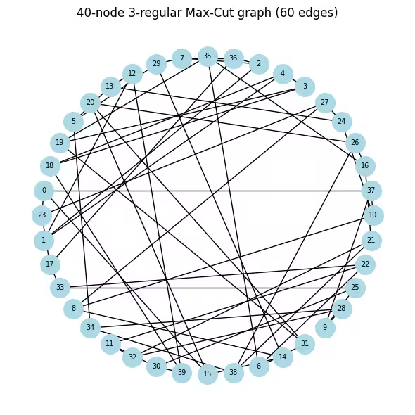
# A 3-regular graph (every node has exactly 3 neighbors) is a standard QAOA
N_LARGE = 40
G_large = nx.random_regular_graph(d=3, n=N_LARGE, seed=0)
edges_large = list(G_large.edges())
print(f"Graph: {N_LARGE} nodes, {len(edges_large)} edges (3-regular)")

# Visualize the graph so it is clear what problem we are solving before any
# quantum work. Nodes in a circular layout; each edge contributes +1 to the
# cut value when its endpoints land in different partitions.
pos_large = nx.circular_layout(G_large)
fig, ax = plt.subplots(figsize=(6, 6))
nx.draw(
    G_large,
    pos_large,
    with_labels=True,
    node_color="lightblue",
    node_size=400,
    font_size=7,
    ax=ax,
)
ax.set_title(f"40-node 3-regular Max-Cut graph ({len(edges_large)} edges)")
plt.tight_layout()
plt.show()

# Same Maxcut → OptimizationProblem → QUBO → Ising pipeline as the small example,
# applied to the 40-node graph.
prob_large = Maxcut(G_large).to_optimization_problem()
converter_large = OptimizationProblemToQubo()
qubo_large = converter_large.convert(prob_large)
cost_op_large, offset_large = to_ising(qubo_large)
n_qubits_large = cost_op_large.num_qubits
print(
    f"Cost operator: {n_qubits_large} qubits, {len(cost_op_large)} Pauli terms"
)

# ── Step 1b: QP relaxation (multi-start L-BFGS-B) ─────────────────────────
# Same multi-start approach as the small example. At 40 qubits the relaxed
# landscape has many more local minima, so 200 random starts are essential
# to find a low-energy warm-start point.
Q_large = qubo_large.objective.quadratic.to_array(symmetric=True)
mu_large = qubo_large.objective.linear.to_array()

def qp_obj_large(x):
    return x @ Q_large @ x + mu_large @ x + qubo_large.objective.constant

bounds_large = [(0.0, 1.0)] * n_qubits_large
rng_qp = np.random.default_rng(42)
best_val_large, c_star_large = np.inf, None

for _ in range(200):
    x0 = rng_qp.uniform(0.0, 1.0, n_qubits_large)
    res = minimize(qp_obj_large, x0, method="L-BFGS-B", bounds=bounds_large)
    if res.fun < best_val_large:
        best_val_large, c_star_large = res.fun, res.x

# Regularize and convert to rotation angles (same formula as small example)
epsilon_large = 0.25
c_clipped_large = np.clip(c_star_large, epsilon_large, 1 - epsilon_large)
thetas_large = 2 * np.arcsin(np.sqrt(c_clipped_large))
print(
    f"c* range: [{c_star_large.min():.3f}, {c_star_large.max():.3f}]  "
    f"theta range: [{thetas_large.min():.3f}, {thetas_large.max():.3f}] rad"
)

# Plot the distribution of c* values to see how much structure the relaxation
# extracted. Values near 0/1 mean confident assignments; values near 0.5 mean
# the classical solver was uncertain and quantum exploration is most needed there.
fig, ax = plt.subplots(figsize=(6, 3))
ax.hist(c_star_large, bins=20, color="steelblue", edgecolor="white")
ax.axvline(0.5, color="k", linestyle="--", label="Uniform prior (std QAOA)")
ax.set_xlabel(r"$c^*_i$")
ax.set_ylabel("Count")
ax.set_title(r"Distribution of warm-start values $c^*_i$ (40-node graph)")
ax.legend()
plt.tight_layout()
plt.show()

# ── Step 1c: Build WS-QAOA circuit ─────────────────────────────────────────
# Reuse build_ws_qaoa from the small-scale section unchanged; the helper
# scales automatically with n_qubits and the cost operator size.
p_large = 1
ws_qc_large, ws_gammas_large, ws_betas_large = build_ws_qaoa(
    cost_op_large, p_large, n_qubits_large, thetas_large
)
ws_qc_large.measure_all()

# ── Step 2: Transpile to hardware-native gates ──────────────────────────
# generate_preset_pass_manager compiles the abstract circuit to th
# gate set of the backend and inserts SWAP gates wherever the cost Hamiltonian
# couples qubits that are not directly connected on the processor.
pm = generate_preset_pass_manager(optimization_level=3, backend=backend)
ws_isa_large = pm.run(ws_qc_large)

ecr_count = ws_isa_large.count_ops().get("ecr", 0)
print(
    f"\nTranspiled circuit: 2Q depth={ws_isa_large.depth(lambda x: x.operation.num_qubits == 2)}"
)
ws_isa_large.draw("mpl", fold=-1)

Graph: 40 nodes, 60 edges (3-regular)

Cost operator: 40 qubits, 60 Pauli terms
c* range: [0.000, 1.000]  theta range: [1.047, 2.094] rad

Transpiled circuit: 2Q depth=86

# ── Classical baseline via simulated annealing ────────────────────
# Run SA before any hardware calls to get a strong classical reference cut
# value. SA is fast (seconds), needs no solver license, and reliably finds
# near-optimal solutions on 40-node graphs. We use sa_cut as the denominator
# for the approximation ratio instead of the looser QP upper bound.
#
# At each step we flip a random node and accept the move if it improves the
# cut, or with probability exp(delta/T) otherwise. Temperature T decays
# geometrically, allowing uphill moves early on to escape local minima.
def simulated_annealing_maxcut(
    G, seed=0, T0=2.0, T_min=1e-4, alpha=0.995, n_steps=100_000
):
    rng_sa = np.random.default_rng(seed)
    n = G.number_of_nodes()
    x = rng_sa.integers(0, 2, n)
    best_x = x.copy()
    best_cut = sum(1 for u, v in G.edges() if x[u] != x[v])
    T = T0
    for _ in range(n_steps):
        i = rng_sa.integers(0, n)
        delta = sum((-1 if x[i] != x[nb] else 1) for nb in G.neighbors(i))
        if delta > 0 or rng_sa.random() < np.exp(delta / T):
            x[i] ^= 1
            cut = sum(1 for u, v in G.edges() if x[u] != x[v])
            if cut > best_cut:
                best_cut, best_x = cut, x.copy()
        T = max(T * alpha, T_min)
    return best_x, best_cut

sa_solution, sa_cut = simulated_annealing_maxcut(G_large)
print(f"Simulated annealing cut value: {sa_cut}  (classical reference)")

# ── Step 3: Execution on hardware ───────────────────────────
# A Session reserves the backend so the COBYLA iterations and final sampling
# run back-to-back without re-queuing between jobs — important when the
# optimizer submits many short jobs sequentially. All jobs are tagged with
# "TUT_WSQAOA" for traceability in the IBM Quantum dashboard.
#
# EstimatorV2 with resilience_level=1 enables twirled readout error extinction
# (TREX), which corrects systematic measurement bit-flip errors without extra
# circuit overhead. 4096 shots per call balances estimation noise vs. job time.
estimator_options = EstimatorOptions()
estimator_options.resilience_level = 1
estimator_options.default_shots = 4096
estimator_options.environment.job_tags = ["TUT_WSQAOA"]

# Align the cost observable with the physical qubit layout chosen by the transpiler
cost_op_isa = cost_op_large.apply_layout(ws_isa_large.layout)
ws_param_order_isa = list(ws_isa_large.parameters)

ws_history_hw = []

with Session(backend=backend) as session:
    estimator_hw = Estimator(mode=session, options=estimator_options)

    def hw_cost_fn(params):
        bound = ws_isa_large.assign_parameters(
            dict(zip(ws_param_order_isa, params))
        )
        energy = (
            estimator_hw.run([(bound, cost_op_isa)]).result()[0].data.evs.real
        )
        ws_history_hw.append(float(energy))
        print(
            f"  iter {len(ws_history_hw):>3d}  <H_C> = {energy:.4f}", end="\r"
        )
        return float(energy)

    # Warm-start initialization: gamma=0 means the cost unitary is the identity on
    # the first call, so COBYLA immediately evaluates the warm-start state itself —
    # a much better starting signal than a random point.
    ws_params0_hw = np.concatenate(
        [np.zeros(p_large), np.full(p_large, np.pi / 4)]
    )

    ws_result_hw = minimize(
        hw_cost_fn,
        ws_params0_hw,
        method="COBYLA",
        options={"maxiter": 150, "rhobeg": 0.3},
    )
    print(
        f"\nOptimization complete: energy={ws_result_hw.fun:.4f}, "
        f"iterations={len(ws_history_hw)}"
    )

    # ── Step 3b: Sample the optimized circuit ──────────────────────────────────
    # Use 8192 shots for the final sample to get a reliable mode estimate.
    sampler_hw = Sampler(
        mode=session,
        options={"environment": {"job_tags": ["TUT_WSQAOA"]}},
    )
    ws_bound_hw = ws_isa_large.assign_parameters(
        dict(zip(ws_param_order_isa, ws_result_hw.x))
    )
    counts_hw = (
        sampler_hw.run([ws_bound_hw], shots=8192)
        .result()[0]
        .data.meas.get_counts()
    )

best_bs_hw = max(counts_hw, key=counts_hw.get)
best_count = counts_hw[best_bs_hw]
total_shots = sum(counts_hw.values())

# Decode: Qiskit returns bitstrings with qubit 0 at the rightmost position,
# so reversing the string maps character index i to variable x_i.
cut_val_hw, s0_hw, s1_hw = evaluate_cut(best_bs_hw[::-1], G_large)

# Compare against simulated annealing.
# A ratio >= 1.0 means WS-QAOA matched or beat the classical SA solution.
# A ratio close to 1.0 (e.g. > 0.95) shows the quantum result is competitive.
approx_ratio_hw = cut_val_hw / sa_cut
print(
    f"Most-probable bitstring frequency: {best_count}/{total_shots} "
    f"({100*best_count/total_shots:.1f}%)"
)
print(
    f"WS-QAOA cut: {cut_val_hw}  |  SA cut: {sa_cut}  "
    f"|  Approximation ratio vs SA: {approx_ratio_hw:.4f}"
)

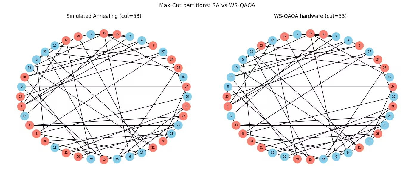
# Visualize both solutions side-by-side on the graph.
# Blue = partition S, orange = partition S-bar.
# Edges crossing between colors are the ones counted in the cut.
fig, axes = plt.subplots(1, 2, figsize=(14, 6))
for ax, assignment, cut, title in [
    (
        axes[0],
        list(sa_solution),
        sa_cut,
        f"Simulated Annealing (cut={sa_cut})",
    ),
    (
        axes[1],
        [int(b) for b in best_bs_hw[::-1]],
        cut_val_hw,
        f"WS-QAOA hardware (cut={cut_val_hw})",
    ),
]:
    colors = [
        "skyblue" if assignment[i] == 0 else "salmon" for i in G_large.nodes()
    ]
    nx.draw(
        G_large,
        pos_large,
        with_labels=True,
        node_color=colors,
        node_size=400,
        font_size=7,
        ax=ax,
    )
    ax.set_title(title)
plt.suptitle("Max-Cut partitions: SA vs WS-QAOA", fontsize=13)
plt.tight_layout()
plt.show()

# ── Step 4: Convergence plot and summary ──────────────────────────────────
# On real hardware the trace will be noisy (shot noise + gate errors), but the
# overall downward trend confirms that COBYLA is making progress despite noise.
fig, ax = plt.subplots(figsize=(7, 4))
ax.plot(ws_history_hw, color="tab:orange", label="WS-QAOA (hardware)")
ax.axhline(
    ws_result_hw.fun,
    color="tab:orange",
    linestyle=":",
    label=f"Final energy ({ws_result_hw.fun:.3f})",
)
ax.set_xlabel("Optimizer call")
ax.set_ylabel(r"$\langle H_C \rangle$")
ax.set_title(f"WS-QAOA convergence on {backend.name} (40 qubits, p=1)")
ax.legend()
plt.tight_layout()
plt.show()

print("\n=== Large Scale Summary ===")
print(f"{'Metric':<38} {'Value':>10}")
print("-" * 50)
print(f"{'Nodes / Edges':<38} {N_LARGE:>5} / {len(edges_large):<4}")
print(f"{'QAOA layers (p)':<38} {p_large:>10}")
print(f"{'Transpiled ECR gate count':<38} {ecr_count:>10}")
print(f"{'Transpiled circuit depth':<38} {ws_isa_large.depth():>10}")
print(f"{'Optimizer iterations':<38} {len(ws_history_hw):>10}")
print(f"{'WS-QAOA energy (hardware)':<38} {ws_result_hw.fun:>10.4f}")
print(f"{'Cut value':<38} {cut_val_hw:>10}")
print(f"{'Simulated annealing cut value':<38} {sa_cut:>10}")
print(f"{'Approximation ratio (vs SA)':<38} {approx_ratio_hw:>10.4f}")

Simulated annealing cut value: 53  (classical reference)
  iter  31  <H_C> = -12.4094
Optimization complete: energy=-13.0256, iterations=31
Most-probable bitstring frequency: 4/8192 (0.0%)
WS-QAOA cut: 53  |  SA cut: 53  |  Approximation ratio vs SA: 1.0000

=== Large Scale Summary ===
Metric                                      Value
--------------------------------------------------
Nodes / Edges                             40 / 60  
QAOA layers (p)                                 1
Transpiled ECR gate count                       0
Transpiled circuit depth                      276
Optimizer iterations                           31
WS-QAOA energy (hardware)                -13.0256
Cut value                                      53
Simulated annealing cut value                  53
Approximation ratio (vs SA)                1.0000

Наступні кроки

Рекомендації

Якщо ця робота видалася тобі цікавою, тебе можуть зацікавити такі матеріали:

• Більше шарів QAOA: збільш p, щоб побачити, як обидва алгоритми покращуються з більшою кількістю шарів схеми, і чи зберігається перевага WS-QAOA за малої глибини.
• Аддон Qiskit optimization mapper: досліди документацію і спробуй змоделювати інші комбінаторні задачі або використати інші розв'язувачі для неперервної релаксації.

Посилання

[1] D. J. Egger, J. Mareček, and S. Woerner, "Warm-starting quantum optimization," Quantum, vol. 5, p. 479, 2021. arXiv:2009.10095

[2] E. Farhi, J. Goldstone, and S. Gutmann, "A quantum approximate optimization algorithm," arXiv:1411.4028, 2014.