Симуляція розсіювання нейтронів у квантових матеріалах за допомогою квантових схем

Оцінка часу використання: 13 хвилин на процесорі Heron r2 (ПРИМІТКА: це лише оцінка. Твій фактичний час виконання може відрізнятися.)

Який туторіал варто використати?

Використай цей туторіал, щоб вивчити реалізацію крок за кроком, із класичними обчисленнями, що виконуються локально на твоєму ноутбуці, та апаратним виконанням на QPU IBM Quantum®. Великомасштабний приклад вимагає значної кількості пам'яті, а наближена квантова компіляція (AQC) може займати кілька годин на типових ресурсах ноутбука. Щоб перекласти стиснення на обчислювальні й пам'яттєві ресурси Qiskit Serverless, скористайся супутнім туторіалом Serverless.

Результати навчання

Як спектри непружного розсіювання нейтронів (INS) пов'язані з динамічними структурними факторами (DSF) квантових спінових моделей.
Як підготувати основний стан, застосувати локальне збурення та виконати часову еволюцію Троттера на квантовій схемі.
Як використовувати наближене квантове компілювання (AQC) з qiskit-addon-aqc-tensor для стиснення глибоких схем Троттера для виконання на апаратному забезпеченні.
Як отримати запізнілу функцію Гріна (RGF) із очікуваних значень кубітів та перетворити її за Фур'є в DSF.

Передумови

Теоретичні відомості

У цьому туторіалі ми відтворюємо результати Lee et al., arXiv:2603.15608.

Розсіювання нейтронів допомагає дослідникам характеризувати матеріали, актуальні для сталого розвитку, зокрема електроди акумуляторів. Цей посібник досліджує, як квантові схеми можуть моделювати магнітні збудження та пов'язувати теоретичні моделі з вимірюваннями розсіювання. Його приклад квантового магніту розвиває методи вивчення поведінки матеріалів, доповнюючи ширший дослідницький інструментарій для відкриття матеріалів.

Непружне розсіювання нейтронів і динамічний структурний фактор

Непружне розсіювання нейтронів (INS) — один з найпотужніших експериментальних методів дослідження магнітних збуджень у квантових матеріалах. Коли пучок теплових або холодних нейтронів потрапляє на кристал, окремі нейтрони обмінюються імпульсом $\mathbf{q}$ та енергією $\omega$ з магнітною підсистемою. Виміряна інтенсивність розсіювання пропорційна динамічному структурному фактору (DSF),

$S^{\alpha\beta}(q,\omega) = \sum_{j} e^{-iq\,j}\int_{-\infty}^{\infty} dt\; e^{i\omega t}\, \langle S_0^{\alpha}(0)\, S_j^{\beta}(t)\rangle,$

який кодує повні просторово-часові кореляції спінових ступенів вільності.

KCuF $_3$ : канонічний магнетик Латтінжерівської рідини

Фторид міді-калію (KCuF $_3$ ) — квазіодновимірний антиферомагнетик, у якому ланцюжки іонів Cu $^{2+}$ зі спіном $\frac{1}{2}$ взаємодіють через обмінну взаємодію Гейзенберга $J$ між найближчими сусідами, тоді як міжланцюжкова взаємодія становить лише $\sim 2.7\%$ від $J$ . При $T = 6\;\mathrm{K}$ , для якої доступні дані INS, спектр домінується фракціоналізованими спінонними збудженнями, характерними для рідини Томонаги-Латтінжера. Оскільки внутрішньоланцюжкова динаміка добре описується одновимірним гамільтоніаном XXZ зі спіном $\frac{1}{2}$ в ізотропній точці ( $\epsilon = 1$ ),

$H = J\sum_{i}\left[S_i^Z S_{i+1}^Z + \epsilon\left(S_i^X S_{i+1}^X + S_i^Y S_{i+1}^Y\right)\right],$

KCuF $_3$ слугує ідеальним еталоном для квантового моделювання: гамільтоніан достатньо простий, щоб реалізувати його на квантовому процесорі, проте основний стан сильно заплутаний, а спектр збуджень містить широкий двоспіноновий континуум.

Примітка: у цьому туторіалі за одиницю енергії взято $J = 1$ і використано нормалізацію $H = J\sum_i[\ldots]$ , що відповідає локальному гамільтоніану $H_\mathrm{loc} = J(S^X S^X + S^Y S^Y + S^Z S^Z)$ , використаному в реалізації схеми зі статті (рис. S3 додаткових матеріалів). Повний гамільтоніан статті (рів. 3) має додатковий загальний множник 2, тому $J$ статті вдвічі більший за $J$ , використаний тут.

Що ми моделюємо і вимірюємо

Фізична величина, яку ми обчислюємо, — це запізніла функція Гріна (RGF), визначена як залежна від часу спін-спінова кореляційна функція

$G^R_{\alpha,\beta}(j, j_c, t) = -\frac{i}{2}\,\langle\psi_{\mathrm{GS}}|\,S_j^\alpha(t)\,S_{j_c}^\beta(0) - S_{j_c}^\beta(0)\,S_j^\alpha(t)\,|\psi_{\mathrm{GS}}\rangle,$

де $j_c$ — опорний сайт (центр ланцюжка), а $S_j^\alpha(t) = e^{iHt}S_j^\alpha e^{-iHt}$ — спіновий оператор у картині Гейзенберга. У цьому туторіалі ми зосереджуємося на компоненті $zz$ ( $\alpha = \beta = z$ ). На квантовому комп'ютері RGF отримують, готуючи основний стан, застосовуючи локальне збурення в $j_c$ , еволюціонуючи збурений стан у часі та вимірюючи однокубітове очікуване значення $\langle\sigma_j^z\rangle$ на кожному сайті $j$ для кожного часового кроку. Ключове розуміння полягає в тому, що кожне $\langle\sigma_j^z\rangle$ дає різницю від намагніченості основного стану; оскільки ізотропний антиферомагнетик Гейзенберга має нульову сумарну намагніченість на сайт ( $\langle\sigma_j^z\rangle_\mathrm{GS} = 0$ ), необроблене виміряне значення безпосередньо дає $G^R(j, j_c, t)$ без будь-якого явного віднімання.

Зібравши $G^R(j, j_c, t)$ для всіх сайтів і часових кроків, ми формуємо двовимірний набір даних, який потім перетворюється за Фур'є як за простором, так і за часом, щоб отримати динамічний структурний фактор $S(q,\omega)$ . DSF — це величина, яку безпосередньо вимірюють в експерименті INS: вона показує, які магнітні збудження існують при кожному імпульсі $q$ та енергії $\omega$ . Для ізотропного ланцюжка Гейзенберга точний спектр збуджень — це двоспіноновий континуум, широка смуга інтенсивності розсіювання, форма якої слугує суворим наскрізним еталоном для квантового моделювання: вона одночасно перевіряє підготовку основного стану, збурення, еволюцію в часі методом Троттера та протокол вимірювання.

Робочий процес квантового моделювання

Робочий процес відображає фізику події INS. Ми (1) готуємо багаточастинковий основний стан $|\psi_{\mathrm{GS}}\rangle$ на $n$ кубітах, (2) застосовуємо локальне збурення перевертання спіну $U_{j_c} = \frac{1}{\sqrt{2}}(I - i\sigma^z_{j_c})$ у центрі ланцюжка, щоб імітувати передачу спіну нейтрона, (3) еволюціонуємо під дією $H$ протягом дискретних часових кроків з використанням троттеризації другого порядку, і (4) вимірюємо $\langle\sigma_i^z\rangle$ на кожному кубіті на кожному кроці, щоб отримати RGF. Двовимірне дискретне перетворення Фур'є потім дає DSF $S(q,\omega)$ .

Спостережувана величина, яку ми вимірюємо на кожному часовому кроці, — це $\sigma_i^z$ на кожному кубіті $i$ . У Qiskit це представлено як список операторів SparsePauliOp: один однокубітовий $Z$ , вбудований у рядок тотожності з $n$ кубітів для кожного сайту. Ці спостережувані величини конструюються один раз для кожного екземпляра задачі під час етапу відображення задачі (крок 1) і повторно використовуються для кожної схеми в цьому масштабі.

Наближена квантова компіляція (AQC)

Глибокі схеми Троттера можна стиснути за допомогою наближеної квантової компіляції (AQC), яка замінює перші кілька шарів Троттера коротшим параметризованим анзацом, параметри якого класично оптимізуються для максимізації точності на рівні MPS відносно оригінальної глибокої схеми. Решта кроків Троттера додаються точно, утворюючи "змішану" схему AQC + Троттер із суттєво меншою кількістю двокубітових вентилів.

Моделювання MPS

Для одновимірної системи методи матрично-добуткового стану (MPS) можуть ефективно моделювати як підготовку основного стану (за допомогою групи ренормалізації матриці густини, або DMRG), так і еволюцію в часі на рівні схеми. Керуючи розмірністю зв'язку $\chi$ , ми обмінюємо точність на обчислювальну вартість. У цьому туторіалі ми використовуємо моделювання MPS у qiskit-addon-aqc-tensor для обчислення високоточних анзаців AQC, які стискають глибокі схеми Троттера для виконання на апаратному забезпеченні.

Вимоги

Перш ніж почати цей туторіал, переконайся, що в тебе встановлено таке:

Qiskit SDK з підтримкою візуалізації
Qiskit Runtime (pip install qiskit-ibm-runtime)
qiskit-addon-aqc-tensor з додатками quimb та JAX (pip install 'qiskit-addon-aqc-tensor[quimb-jax]')

Налаштування

# Added by doQumentation — installs the packages this notebook needs if they are missing
import importlib.util

_needed = {"matplotlib": "matplotlib", "numpy": "numpy", "qiskit": "qiskit", "qiskit_addon_aqc_tensor": "qiskit-addon-aqc-tensor", "qiskit_ibm_runtime": "qiskit-ibm-runtime", "qiskit_quimb": "qiskit-quimb", "quimb": "quimb", "scipy": "scipy"}
_missing = [pip for module, pip in _needed.items()
            if importlib.util.find_spec(module) is None]
# One at a time, so a package that fails to install does not block the others
for _pip in _missing:
    %pip install -q {_pip}
if not _missing:
    print("\u2713 All required packages are installed")

import timeit
import warnings
from collections.abc import Iterator, Sequence
from functools import partial

import matplotlib.pyplot as plt
import numpy as np
import quimb.tensor as qtn
import scipy.optimize
from numpy.typing import NDArray
from qiskit import QuantumCircuit
from qiskit.circuit import CircuitInstruction, ParameterVector, Qubit
from qiskit.circuit.library import PauliEvolutionGate
from qiskit.primitives import StatevectorEstimator
from qiskit.quantum_info import SparsePauliOp
from qiskit.transpiler.preset_passmanagers import generate_preset_pass_manager
from qiskit_addon_aqc_tensor import generate_ansatz_from_circuit
from qiskit_addon_aqc_tensor.objective import MaximizeStateFidelity
from qiskit_addon_aqc_tensor.simulation import tensornetwork_from_circuit
from qiskit_addon_aqc_tensor.simulation.quimb import QuimbSimulator
from qiskit_ibm_runtime import EstimatorV2 as Estimator
from qiskit_ibm_runtime import QiskitRuntimeService
from qiskit_quimb import quimb_circuit
from scipy.sparse import SparseEfficiencyWarning

# scipy.sparse.linalg.expm (reached via PauliEvolutionGate.to_matrix) prefers
# CSC and warns when handed the CSR matrix from SparsePauliOp.to_matrix; the
# result is unaffected, so silence the cosmetic warning.
warnings.filterwarnings("ignore", category=SparseEfficiencyWarning)

def xxz_hamiltonian_mpo(
    n_qubits: int, interaction: float = 1.0, anisotropy: float = 1.0
) -> qtn.MatrixProductOperator:
    """1D XXZ Hamiltonian as a quimb MPO.

    Builds the Hamiltonian using ``qtn.SpinHam1D``.

    Args:
        n_qubits: Number of sites.
        interaction: Overall interaction strength (J in the paper).
        anisotropy: XY/Z anisotropy (ε in the paper). ``ε = 1`` is the
            isotropic Heisenberg point; ``ε = 0`` is the Ising limit.

    Returns:
        The Hamiltonian as a matrix product operator.
    """
    builder = qtn.SpinHam1D(S=1 / 2)
    builder += interaction * anisotropy * 0.5, "+", "-"
    builder += interaction * anisotropy * 0.5, "-", "+"
    builder += interaction, "Z", "Z"
    return builder.build_mpo(L=n_qubits)

def build_ground_state_ansatz(n_qubits: int, n_layers: int) -> QuantumCircuit:
    """Hamiltonian variational ansatz (HVA) circuit for ground-state preparation.

    Starts from a product of singlet pairs and applies alternating
    odd/even layers of parameterized XXZ pair-evolution gates.

    The returned circuit is parameterized: it carries a ``ParameterVector``
    named ``"theta"`` of length ``2 * n_layers`` whose values must be
    assigned (e.g. via ``circuit.assign_parameters``) before simulation.
    Element ``2 * r`` is the odd-layer angle and element ``2 * r + 1`` is the
    even-layer angle of layer ``r``.

    Args:
        n_qubits: Number of qubits (must be even).
        n_layers: Number of HVA layers.

    Returns:
        The parameterized HVA preparation circuit.
    """
    theta = ParameterVector("theta", 2 * n_layers)
    circuit = QuantumCircuit(n_qubits)
    # Initial singlet product state
    for i in range(n_qubits // 2):
        circuit.x(2 * i)
        circuit.x(2 * i + 1)
        circuit.h(2 * i + 1)
        circuit.cx(2 * i + 1, 2 * i)
    # Variational layers: each pair gate is exp(-i theta (XX+YY+ZZ)/2)
    pair_ham = SparsePauliOp(
        ["XX", "YY", "ZZ"], coeffs=[0.5, 0.5, 0.5]
    )  # H_pair (HVA form)
    for r in range(n_layers):
        for i in range(1, (n_qubits + 1) // 2):  # odd layer
            circuit.append(
                PauliEvolutionGate(pair_ham, time=theta[2 * r]),
                [2 * i - 1, 2 * i],
            )
        for i in range(n_qubits // 2):  # even layer
            circuit.append(
                PauliEvolutionGate(pair_ham, time=theta[2 * r + 1]),
                [2 * i, 2 * i + 1],
            )
    return circuit

def optimize_ground_state_ansatz(
    ansatz: QuantumCircuit,
    x0: NDArray[np.floating],
    target_mps: qtn.MatrixProductState,
    *,
    max_bond: int | None = None,
    cutoff: float = 1e-10,
    method: str = "COBYQA",
    options: dict | None = None,
) -> scipy.optimize.OptimizeResult:
    """Optimize HVA parameters by maximizing fidelity with a target MPS.

    The HVA circuit is simulated as a matrix product state with the given
    bond-dimension truncation, and the parameters are optimized to maximize
    the state fidelity ``|<psi_HVA | target_mps>|**2`` with the DMRG ground
    state. Both states are normalized, so the minimized objective is the
    infidelity ``1 - |<psi_HVA | target_mps>|**2``.

    Args:
        ansatz: Parameterized HVA circuit from ``build_ground_state_ansatz``.
            The length of ``x0`` must equal ``ansatz.num_parameters``.
        x0: Initial parameters.
        target_mps: Target MPS (DMRG ground state) to maximize fidelity with.
        max_bond: Maximum MPS bond dimension during gate application.
        cutoff: Singular-value cutoff during gate application.
        method: ``scipy.optimize.minimize`` method.
        options: Options dict forwarded to ``scipy.optimize.minimize``.

    Returns:
        The Scipy OptimizeResult.
    """

    def infidelity(params: NDArray[np.floating]) -> float:
        circuit = ansatz.assign_parameters(params)
        circuit_mps = quimb_circuit(
            circuit.decompose(["PauliEvolution"]),
            quimb_circuit_class=qtn.CircuitMPS,
            max_bond=max_bond,
            cutoff=cutoff,
        )
        return 1 - abs(circuit_mps.psi.H @ target_mps) ** 2

    return scipy.optimize.minimize(
        infidelity, np.asarray(x0), method=method, options=options
    )

def trotter_evolution(
    qubits: Sequence[Qubit],
    interaction: float,
    anisotropy: float,
    time_step: float,
    n_steps: int,
) -> Iterator[CircuitInstruction]:
    """Second-order Trotter steps of the XXZ pair Hamiltonian.

    While the paper used a hand-optimized circuit for the Trotter steps, we use
    PauliEvolutionGate here for simplicity and generality. The final two-qubit gate
    count and gate depth are equivalent when transpiled with ``optimization_level=3``.

    Args:
        qubits: Qubits to act on (length ``n_qubits``).
        interaction: Overall interaction strength (J in the paper).
        anisotropy: XY/Z anisotropy (ε in the paper). ``ε = 1`` is the
            isotropic Heisenberg point; ``ε = 0`` is the Ising limit.
        time_step: Per-step Trotter time.
        n_steps: Number of Trotter steps.

    Yields:
        ``CircuitInstruction``s implementing the Trotter steps.
    """
    if n_steps == 0:
        return
    n_qubits = len(qubits)
    pair_ham = SparsePauliOp(
        ["XX", "YY", "ZZ"],
        coeffs=[
            0.25 * interaction * anisotropy,
            0.25 * interaction * anisotropy,
            0.25 * interaction,
        ],
    )
    half_evo = PauliEvolutionGate(pair_ham, time=time_step / 2)
    full_evo = PauliEvolutionGate(pair_ham, time=time_step)
    for i in range(n_qubits // 2):  # half even layer
        yield CircuitInstruction(half_evo, (qubits[2 * i], qubits[2 * i + 1]))
    for i in range(n_qubits // 2 - 1):  # full odd layer
        yield CircuitInstruction(
            full_evo, (qubits[2 * i + 1], qubits[2 * i + 2])
        )
    for _ in range(n_steps - 1):  # interior steps
        for i in range(n_qubits // 2):
            yield CircuitInstruction(
                full_evo, (qubits[2 * i], qubits[2 * i + 1])
            )
        for i in range(n_qubits // 2 - 1):
            yield CircuitInstruction(
                full_evo, (qubits[2 * i + 1], qubits[2 * i + 2])
            )
    for i in range(n_qubits // 2):  # half even layer
        yield CircuitInstruction(half_evo, (qubits[2 * i], qubits[2 * i + 1]))

def get_dsf(
    n_qubits: int,
    rgf_mat: NDArray[np.floating],
    time_step: float,
    n_steps: int,
    n_points_momentum: int,
    n_points_frequency: int,
) -> NDArray[np.floating]:
    """Compute the dynamical structure factor from the retarded Green's function.

    Uses the center-site approximation and a discrete Fourier transform.
    The result is symmetrized about the momentum axis and clipped to
    non-negative values, ready for plotting.

    Args:
        n_qubits: Number of qubits (sites).
        rgf_mat: RGF matrix of shape ``(n_steps, n_qubits)``.
        time_step: Trotter time-step size.
        n_steps: Number of time steps.
        n_points_momentum: Number of momentum points.
        n_points_frequency: Number of frequency points.

    Returns:
        DSF array of shape ``(n_points_frequency, n_points_momentum)``,
        symmetrized about the momentum axis and clipped to non-negative values.
    """
    max_frequency = np.pi / time_step
    momentum_range = np.linspace(0, 2 * np.pi, n_points_momentum)
    frequency_range = np.linspace(0, max_frequency, n_points_frequency)
    result = np.zeros((frequency_range.shape[0], momentum_range.shape[0]))
    center = n_qubits // 2 - 1
    for iw, w in enumerate(frequency_range):
        exponent = np.exp(1j * w * time_step * np.arange(1, n_steps + 1))
        # S = sigma/2, so two spin operators contribute a factor of (1/2)(1/2) = 1/4.
        rgf_omega = (
            np.dot(rgf_mat.T, exponent) * time_step / 4
        )  # S(omega): time Fourier slice of the Green's function
        for iq, q in enumerate(momentum_range):
            momentum_phases = np.exp(
                -1j * q * np.arange(-center, center + 2, 1)
            )
            result[iw, iq] = np.imag(np.dot(rgf_omega, momentum_phases))
    result = -(result + result[:, ::-1]) / 2
    result = np.clip(result, a_min=0, a_max=None)
    return result

def plot_dsf(
    dsf: NDArray[np.floating],
    time_step: float,
    n_points_momentum: int,
    n_points_frequency: int,
    title: str | None = None,
) -> None:
    """Heat-map of the dynamical structure factor.

    Args:
        dsf: DSF array of shape ``(n_points_frequency, n_points_momentum)``.
        time_step: Trotter time-step size.
        n_points_momentum: Number of momentum points.
        n_points_frequency: Number of frequency points.
        title: Optional plot title.
    """
    max_frequency = np.pi / time_step
    momentum_range = np.linspace(0, 2 * np.pi, n_points_momentum)
    frequency_range = np.linspace(0, max_frequency, n_points_frequency)
    x, y = np.meshgrid(momentum_range, frequency_range)
    fig, ax = plt.subplots(figsize=(8, 5))
    c = ax.pcolormesh(x, y, dsf / np.max(dsf), cmap="viridis", shading="auto")
    fig.colorbar(c, ax=ax, label="Normalized intensity")
    ax.set_ylim(0, 3.6)
    ax.set_xlim(0, 2 * np.pi)
    ax.set_xlabel(r"$q$", fontsize=16)
    ax.set_ylabel(r"$\tilde{\omega} = \omega / J$", fontsize=16)
    ax.set_xticks([0, np.pi / 2, np.pi, 3 * np.pi / 2, 2 * np.pi])
    ax.set_xticklabels(["0", r"$\pi/2$", r"$\pi$", r"$3\pi/2$", r"$2\pi$"])
    if title:
        ax.set_title(title, fontsize=14)
    plt.tight_layout()
    plt.show()

def plot_rgf(
    n_qubits: int,
    rgf_mat: NDArray[np.floating],
    time_step: float,
    n_steps: int,
    title: str | None = None,
) -> None:
    """Heat-map of the retarded Green's function in real space and time.

    Args:
        n_qubits: Number of qubits (sites).
        rgf_mat: RGF matrix of shape ``(n_steps, n_qubits)``.
        time_step: Trotter time-step size.
        n_steps: Number of time steps.
        title: Optional plot title.
    """
    fig, ax = plt.subplots(figsize=(8, 6))
    qubit_axis = np.arange(n_qubits)
    t_axis = np.arange(1, n_steps + 1) * time_step
    x, y = np.meshgrid(qubit_axis, t_axis)
    c = ax.pcolormesh(
        x,
        y,
        np.real(rgf_mat),
        cmap="RdBu",
        vmax=0.5,
        vmin=-0.5,
        shading="auto",
    )
    fig.colorbar(c, ax=ax, label=r"Re $G^R(j, j_c, t)$")
    ax.set_xlabel("Qubit", fontsize=16)
    ax.xaxis.set_major_locator(
        plt.matplotlib.ticker.MaxNLocator(integer=True)
    )
    ax.set_ylabel(r"Time", fontsize=16)
    if title:
        ax.set_title(title, fontsize=14)
    plt.tight_layout()
    plt.show()

def uniform_2q_depth(circuit: QuantumCircuit) -> int:
    """Two-qubit gate depth in a standardized basis."""
    pass_manager = generate_preset_pass_manager(
        optimization_level=0, basis_gates=["cz", "id", "rz", "sx", "x"]
    )
    return pass_manager.run(circuit).depth(
        lambda inst: inst.operation.num_qubits == 2
    )

Приклад для симулятора малого масштабу

Спочатку ми демонструємо повний робочий процес на 10 кубітах, оптимізуючи анзац основного стану HVA за допомогою моделювання MPS та використовуючи симулятор вектора стану Qiskit для еволюції в часі. DMRG дає еталонну енергію основного стану та еталонний MPS. Цей приклад малого масштабу дозволяє перевірити кожен крок перед масштабуванням.

Крок 1: відображення класичних вхідних даних на квантову задачу

Ми починаємо з визначення фізичної моделі та побудови квантових схем.

Гамільтоніан. KCuF $_3$ моделюється 1D гамільтоніаном XXZ в ізотропній точці ( $J = 1$ , $\epsilon = 1$ , взявши $J = 1$ за одиницю енергії).

Основний стан. Ми використовуємо схему гамільтоніан-варіаційного анзацу (HVA), build_ground_state_ansatz, як схему підготовки основного стану. Параметри HVA оптимізуються класично шляхом максимізації точності стану $|\langle\psi_{\mathrm{HVA}}(\theta)|\psi_{\mathrm{DMRG}}\rangle|^2$ з MPS основного стану DMRG, де стан HVA обчислюється шляхом моделювання схеми як матрично-добуткового стану за допомогою CircuitMPS з quimb. Ми використовуємо scipy.optimize.minimize для оптимізації. Енергія $\langle H \rangle$ оптимізованого анзацу також обчислюється для довідки.

Вентилі Троттера. Кожен член взаємодії найближчих сусідів $e^{-i\Delta t\, H_{\mathrm{pair}}}$ з $H_{\mathrm{pair}} = (J/4)(XX + YY + ZZ)$ конструюється за допомогою PauliEvolutionGate(H_pair, time=time_step). Qiskit синтезує це в оптимальну декомпозицію з трьома CNOT під час транспіляції.

Збурення. Вентиль $R_z(\pi/2)$ на центральному кубіті реалізує $U_{j_c} = \frac{1}{\sqrt{2}}(I - i\sigma^z_{j_c})$ , імітуючи локальне перевертання спіну, спричинене розсіяним нейтроном.

Спостережувані величини. Ми конструюємо спостережувану величину $\sigma^z$ для кожного сайту кубіта. Ці об'єкти SparsePauliOp передаються примітиву Estimator на кроці 3 для отримання $\langle\sigma_i^z\rangle$ на кожному часовому кроці.

# -- Physical parameters --
n_qubits = 10
interaction = 1.0  # J
anisotropy = 1.0  # ε (isotropic point)
time_step = 0.6
n_steps = 10
mps_max_bond = 32
mps_cutoff = 1e-8
center = n_qubits // 2 - 1

# -- Hamiltonian MPO --
ham_mpo = xxz_hamiltonian_mpo(n_qubits, interaction, anisotropy)

# -- Reference ground-state energy via DMRG --
dmrg = qtn.DMRG2(ham_mpo)
dmrg.solve(tol=1e-8)
print(f"Ground-state energy (DMRG): {dmrg.energy:.6f}")

# -- Build ground state ansatz circuit --
gs_n_layers = 3
gs_ansatz = build_ground_state_ansatz(n_qubits, gs_n_layers)

# -- Optimize ground state ansatz parameters to maximize fidelity with the DMRG MPS --
# Initialize odd-layer angles near 0 (where the inter-pair gate is the
# identity) and even-layer angles near pi/2 (where the intra-pair gate
# is a SWAP, since 0.5*(XX + YY + ZZ) = SWAP - I/2).
rng = np.random.default_rng(12345)
x0 = np.tile([0, np.pi / 2], gs_n_layers) + rng.normal(
    scale=0.1, size=2 * gs_n_layers
)
print("Optimizing ground state ansatz...")
t0 = timeit.default_timer()
result = optimize_ground_state_ansatz(
    gs_ansatz,
    x0,
    dmrg.state,
    max_bond=mps_max_bond,
    cutoff=mps_cutoff,
    options=dict(maxiter=100),
)
t1 = timeit.default_timer()
print(f"Finished optimizing ground state ansatz in {t1 - t0} seconds.")
print(f"Ground state ansatz fidelity: {1 - result.fun:.6f}")

gs_circuit = gs_ansatz.assign_parameters(result.x)
gs_circuit_mps = quimb_circuit(
    gs_circuit.decompose(["PauliEvolution"]),
    quimb_circuit_class=qtn.CircuitMPS,
    max_bond=mps_max_bond,
    cutoff=mps_cutoff,
)
gs_ansatz_energy = qtn.expec_TN_1D(
    gs_circuit_mps.psi.H, ham_mpo, gs_circuit_mps.psi
)
print(f"Ground state ansatz energy: {gs_ansatz_energy:.6f}")

# -- Build circuits for each time step --
perturbed = gs_circuit.copy()
perturbed.rz(np.pi / 2, center)

circuits = []
for t in range(1, n_steps + 1):
    circuit = perturbed.copy()
    for instr in trotter_evolution(
        circuit.qubits, interaction, anisotropy, time_step, t
    ):
        circuit.append(instr)
    circuits.append(circuit)
print(
    f"Built {len(circuits)} circuits, deepest 2q depth (uniform basis) = "
    f"{uniform_2q_depth(circuits[-1])}"
)

# -- Observables: Z on each qubit site --
observables = [
    SparsePauliOp.from_sparse_list([("Z", [i], 1)], num_qubits=n_qubits)
    for i in range(n_qubits)
]
print(f"Defined {len(observables)} Z observables.")

Ground-state energy (DMRG): -4.258035
Optimizing ground state ansatz...
Finished optimizing ground state ansatz in 8.850687621976249 seconds.
Ground state ansatz fidelity: 0.984277
Ground state ansatz energy: -4.232565
Built 10 circuits, deepest 2q depth (uniform basis) = 163
Defined 10 Z observables.

Крок 2: оптимізація задачі для виконання на квантовому апаратному забезпеченні

Для реального апаратного забезпечення наведені вище схеми Троттера були б занадто глибокими. Наближена квантова компіляція (AQC) вирішує цю проблему, замінюючи перші $k$ шарів Троттера (включно зі схемою основного стану) коротшим параметризованим анзацом, оптимізованим для максимізації точності на рівні MPS відносно оригінальної глибокої схеми. Решта кроків Троттера додаються точно, утворюючи мілкішу схему "AQC + Троттер".

Щоб збалансувати виразність і глибину схеми, використовуються два анзаци: одношаровий анзац (згенерований з одного кроку Троттера) стискає найраніші часові кроки, а глибший двошаровий анзац (згенерований з двох кроків Троттера) стискає наступні кілька кроків, де потрібна вища точність.

Робочий процес AQC складається з чотирьох підкроків:

Побудова цільових схем — перші $k_1 + k_2$ схем з кроку 1 слугують безпосередньо цілями AQC.
Обчислення цільового MPS — моделювання кожної цільової схеми як матрично-добуткового стану за допомогою quimb.tensor.CircuitMPS.
Генерація та оптимізація анзаців — generate_ansatz_from_circuit створює одношаровий та двошаровий параметризовані анзаци; параметри оптимізуються за допомогою L-BFGS-B з градієнтами, прискореними JAX, для мінімізації $1 - |\langle\psi_{\mathrm{ansatz}}|\psi_{\mathrm{target}}\rangle|^2$ . Перші $k_1$ кроків використовують одношаровий анзац, а наступні $k_2$ кроків — двошаровий анзац; у межах кожного етапу кожен крок стартує з оптимізованих параметрів попереднього кроку, а параметри скидаються до значень за замовчуванням етапу на межі етапів.
Складання змішаних схем — для часових кроків після контрольної точки AQC точні шари Троттера додаються до оптимізованої дворівневої схеми AQC за допомогою trotter_evolution.

# Number of time steps to compress into an AQC ansatz with one layer
aqc_n_steps_1 = 3
# Number of time steps to compress into an AQC ansatz with two layers
aqc_n_steps_2 = 2
aqc_n_steps_total = aqc_n_steps_1 + aqc_n_steps_2

# ── Step 2a: Target circuits (first aqc_n_steps_total circuits from Step 1) ──
target_circuits = {
    k: circuits[k - 1] for k in range(1, aqc_n_steps_total + 1)
}
# ── Step 2b: Compute target MPS ──
# Decompose PauliEvolutionGate to RXX/RYY/RZZ before passing to the AQC MPS
# backend, which does not understand PauliEvolutionGate natively.
aqc_sim = QuimbSimulator(
    quimb_circuit_factory=partial(
        qtn.CircuitMPS,
        gate_opts=dict(max_bond=mps_max_bond, cutoff=mps_cutoff),
    ),
    autodiff_backend="jax",
)
print("\nStep 2b — target MPS:")
target_mps = {}
for k in range(1, aqc_n_steps_total + 1):
    target_mps[k] = tensornetwork_from_circuit(
        target_circuits[k].decompose(["PauliEvolution"]), aqc_sim
    )
    print(f"  k={k}: max bond = {target_mps[k].psi.max_bond()}")

# ── Step 2c: Generate ansätze (one-layer and two-layer) and optimize parameters ──
ansatz_1, initial_params_1 = generate_ansatz_from_circuit(
    target_circuits[1].decompose(["PauliEvolution"]),
    qubits_initially_zero=True,
)
initial_params_1 = np.array(initial_params_1)
ansatz_2, initial_params_2 = generate_ansatz_from_circuit(
    target_circuits[2].decompose(["PauliEvolution"]),
    qubits_initially_zero=True,
)
initial_params_2 = np.array(initial_params_2)
print(
    f"\nStep 2c — one-layer ansatz: {ansatz_1.num_parameters} parameters, "
    f"2q depth (uniform basis) = {uniform_2q_depth(ansatz_1)}"
)
print(
    f"Step 2c — two-layer ansatz: {ansatz_2.num_parameters} parameters, "
    f"2q depth (uniform basis) = {uniform_2q_depth(ansatz_2)}"
)

aqc_circuits = {}
aqc_params = {}
for k in range(1, aqc_n_steps_total + 1):
    if k <= aqc_n_steps_1:
        ansatz, base_params = ansatz_1, initial_params_1
    else:
        ansatz, base_params = ansatz_2, initial_params_2
    # Warm-start from the previous step only within the same stage
    same_stage = (k - 1 >= 1) and (
        (k - 1 <= aqc_n_steps_1) == (k <= aqc_n_steps_1)
    )
    x0 = aqc_params[k - 1] if same_stage else base_params
    obj = MaximizeStateFidelity(target_mps[k], ansatz, aqc_sim)
    t0 = timeit.default_timer()
    result = scipy.optimize.minimize(
        obj.loss_function,
        x0,
        method="L-BFGS-B",
        jac=True,
        options=dict(maxiter=100),
    )
    elapsed = timeit.default_timer() - t0
    aqc_params[k] = result.x
    aqc_circuits[k] = ansatz.assign_parameters(result.x)
    print(
        f"  k={k}: fidelity = {1 - result.fun:.4f}, "
        f"2q depth (uniform basis) = "
        f"{uniform_2q_depth(aqc_circuits[k])}, "
        f"{elapsed:.1f}s"
    )

# ── Step 2d: Assemble full circuit set (AQC + Trotter) ──
all_circuits = []
for k in range(1, aqc_n_steps_total + 1):
    all_circuits.append(aqc_circuits[k])
base = aqc_circuits[aqc_n_steps_total]
for k in range(1, n_steps - aqc_n_steps_total + 1):
    circuit = base.copy()
    for instr in trotter_evolution(
        circuit.qubits, interaction, anisotropy, time_step, k
    ):
        circuit.append(instr)
    all_circuits.append(circuit)

full_depths = [
    uniform_2q_depth(circuits[k - 1]) for k in range(1, n_steps + 1)
]
aqc_depths = [uniform_2q_depth(circuit) for circuit in all_circuits]
full_2q = [
    circuits[k - 1].decompose(["PauliEvolution"]).num_nonlocal_gates()
    for k in range(1, n_steps + 1)
]
aqc_2q = [
    circuit.decompose(["PauliEvolution"]).num_nonlocal_gates()
    for circuit in all_circuits
]
print(f"\nStep 2d — assembled {len(all_circuits)} circuits")
print(
    f"  At step {n_steps} (uniform basis): "
    f"Trotter 2q depth = {full_depths[-1]}, AQC+Trotter 2q depth = {aqc_depths[-1]}; "
    f"2q gates: Trotter = {full_2q[-1]}, AQC+Trotter = {aqc_2q[-1]}"
)

steps_axis = np.arange(1, n_steps + 1)
fig, ax = plt.subplots(figsize=(7, 4))
ax.plot(steps_axis, full_depths, "-o", color="black", label="Full Trotter")
ax.plot(
    steps_axis, aqc_depths, "-o", color="cadetblue", label="AQC + Trotter"
)
ax.set_xlabel("Trotter steps", fontsize=13)
ax.xaxis.set_major_locator(plt.matplotlib.ticker.MaxNLocator(integer=True))
ax.set_ylabel("2q gate depth (uniform basis)", fontsize=13)
ax.set_title(f"AQC circuit-depth reduction ({n_qubits} qubits)", fontsize=13)
ax.legend(fontsize=11)
plt.tight_layout()
plt.show()

Step 2b — target MPS:
  k=1: max bond = 22
  k=2: max bond = 22
  k=3: max bond = 26
  k=4: max bond = 27
  k=5: max bond = 30

Step 2c — one-layer ansatz: 389 parameters, 2q depth (uniform basis) = 27
Step 2c — two-layer ansatz: 470 parameters, 2q depth (uniform basis) = 33
  k=1: fidelity = 1.0000, 2q depth (uniform basis) = 27, 11.8s
  k=2: fidelity = 0.9980, 2q depth (uniform basis) = 27, 13.2s
  k=3: fidelity = 0.9890, 2q depth (uniform basis) = 27, 13.7s
  k=4: fidelity = 0.9983, 2q depth (uniform basis) = 33, 16.4s
  k=5: fidelity = 0.9957, 2q depth (uniform basis) = 33, 16.4s

Step 2d — assembled 10 circuits
  At step 10 (uniform basis): Trotter 2q depth = 163, AQC+Trotter 2q depth = 99; 2q gates: Trotter = 371, AQC+Trotter = 200

Output of the previous code cell

Крок 3: виконання за допомогою примітивів Qiskit

Ми моделюємо кожну скомпільовану AQC схему за допомогою примітиву StatevectorEstimator.

estimator = StatevectorEstimator()
pubs = [(circuit, observables) for circuit in all_circuits]
job = estimator.run(pubs)
result = job.result()

Крок 4: постобробка та повернення результату в потрібному класичному форматі

Тепер ми отримуємо очікуване значення $\langle\sigma_i^z\rangle$ для кожного кубіта $i$ на кожному часовому кроці $t$ . Ці значення утворюють матрицю запізнілої функції Гріна $G^R(j, j_c, t)$ . Потім ми перетворюємо RGF за Фур'є в динамічний структурний фактор $S(q, \omega)$ і будуємо графіки як RGF, так і DSF. get_dsf внутрішньо застосовує дзеркальну симетрію та обрізає від'ємні значення.

rgf_mat = np.stack([pub_result.data.evs for pub_result in result])

# -- Compute DSF --
n_points_momentum, n_points_frequency = 100, 100
spectrum = get_dsf(
    n_qubits,
    rgf_mat,
    time_step,
    n_steps,
    n_points_momentum,
    n_points_frequency,
)

# -- Plot retarded Green's function --
plot_rgf(
    n_qubits,
    rgf_mat,
    time_step,
    n_steps,
    title=f"Retarded Green's function — {n_qubits} qubits (simulation)",
)

# -- Plot DSF --
plot_dsf(
    spectrum,
    time_step,
    n_points_momentum,
    n_points_frequency,
    title=f"Dynamical structure factor — {n_qubits} qubits (simulation)",
)

Output of the previous code cell

Виконання на апаратному забезпеченні великого масштабу

Тепер ми масштабуємося до 50 кубітів. У цьому масштабі оптимізації досягають нижчих точностей, ніж у прикладі малого масштабу: точність анзацу основного стану падає приблизно до 0.65, а точності AQC знижуються приблизно до 0.7 на пізніших контрольних точках. Це очікувано, і ти можеш покращити ці точності, збільшивши кількість шарів анзацу основного стану (gs_n_layers) або кількість ітерацій оптимізації (maxiter) за додаткову класичну вартість. Зверни також увагу, що точності двошарового AQC виявляються нижчими, ніж одношарового. Це не регресія: пізніші часові кроки генерують більше заплутаності і їх просто важче стискати, тому для них використовується більш виразний двошаровий анзац.

Оптимізація AQC також може зайняти кілька годин класичного обчислювального часу (приблизно шість годин у запуску, показаному тут, більшість з яких витрачено на дворівневі контрольні точки на кроці 2c). Щоб зменшити фактичний час виконання, розглянь можливість запуску цього блокнота на потужнішому класичному апаратному забезпеченні, наприклад системі високопродуктивних обчислень (HPC). Альтернативно, можеш зменшити масштаб задачі (наприклад, менше кубітів або менше часових кроків); твої результати тоді відрізнятимуться від показаних тут.

Наведений нижче код дотримується тієї ж чотирикрокової структури, що й приклад малого масштабу. Параметри основного стану HVA знову оптимізуються за допомогою моделювання MPS. На QPU ми вмикаємо динамічне розв'язування (DD), твірлінг Паулі та твірлінг-гасіння похибок зчитування (TREX) для придушення та пом'якшення похибок. Наступна таблиця підсумовує, чим експеримент великого масштабу відрізняється від малого:

	Малий масштаб	Великий масштаб
Кубіти	10	50
Часові кроки	10	20
Контрольні точки AQC (1-рівневі + 2-рівневі)	3 + 2 = 5	6 + 4 = 10
Шари анзацу основного стану	3	5
Максимальна розмірність зв'язку MPS	32	128
Estimator	`StatevectorEstimator`	QPU з DD, твірлінгом Паулі та TREX

Повідомлення про повільну компіляцію XLA

Під час оптимізації AQC (крок 2c нижче) ти можеш побачити повідомлення stderr, такі як:

[Compiling module jit_MakeArrayFn for CPU] Very slow compile? ...
The operation took 2m14s

Це нешкідливі діагностичні повідомлення від XLA, компілятора, який лежить в основі автоматичного диференціювання JAX у qiskit-addon-aqc-tensor. При 50 кубітах з розмірністю зв'язку MPS 128 XLA витрачає кілька хвилин на компіляцію функції градієнта під час першого трасування. Компіляція завершується успішно, і результати оптимізації не постраждають.

# ── Parameters ──────────────────────────────────────────────────────────────
n_qubits = 50  # 10 → 50
interaction = 1.0  # J
anisotropy = 1.0  # ε (isotropic point)
time_step = 0.6
n_steps = 20  # 10 → 20
aqc_n_steps_1 = 6  # 3 → 6
aqc_n_steps_2 = 4  # 2 → 4
aqc_n_steps_total = aqc_n_steps_1 + aqc_n_steps_2
gs_n_layers = 5  # 3 → 5
mps_max_bond = 128  # 32 -> 128
mps_cutoff = 1e-8
center = n_qubits // 2 - 1

# ── Step 1: Map ──────────────────────────────────────────────────────────────
ham_mpo = xxz_hamiltonian_mpo(n_qubits, interaction, anisotropy)

dmrg = qtn.DMRG2(ham_mpo)
dmrg.solve(tol=1e-8)
print(f"Ground-state energy (DMRG): {dmrg.energy:.6f}")

gs_ansatz = build_ground_state_ansatz(n_qubits, gs_n_layers)

rng = np.random.default_rng(12345)
x0 = np.tile([0.0, np.pi / 2], gs_n_layers) + rng.normal(
    scale=0.1, size=2 * gs_n_layers
)
print("Optimizing ground state ansatz...")
t0 = timeit.default_timer()
result = optimize_ground_state_ansatz(
    gs_ansatz,
    x0,
    dmrg.state,
    max_bond=mps_max_bond,
    cutoff=mps_cutoff,
    options=dict(maxiter=100),
)
t1 = timeit.default_timer()
print(f"Finished optimizing ground state ansatz in {t1 - t0} seconds.")
print(f"Ground state ansatz fidelity: {1 - result.fun:.6f}")

gs_circuit = gs_ansatz.assign_parameters(result.x)
gs_circuit_mps = quimb_circuit(
    gs_circuit.decompose(["PauliEvolution"]),
    quimb_circuit_class=qtn.CircuitMPS,
    max_bond=mps_max_bond,
    cutoff=mps_cutoff,
)
gs_ansatz_energy = qtn.expec_TN_1D(
    gs_circuit_mps.psi.H, ham_mpo, gs_circuit_mps.psi
)
print(f"Ground state ansatz energy: {gs_ansatz_energy:.6f}")

perturbed = gs_circuit.copy()
perturbed.rz(np.pi / 2, center)

circuits = []
for t in range(1, n_steps + 1):
    circuit = perturbed.copy()
    for instr in trotter_evolution(
        circuit.qubits, interaction, anisotropy, time_step, t
    ):
        circuit.append(instr)
    circuits.append(circuit)
print(
    f"Built {len(circuits)} circuits, deepest 2q depth (uniform basis) = "
    f"{uniform_2q_depth(circuits[-1])}"
)

observables = [
    SparsePauliOp.from_sparse_list([("Z", [i], 1)], num_qubits=n_qubits)
    for i in range(n_qubits)
]
print(f"Defined {len(observables)} Z observables.")

# ── Step 2: AQC ──────────────────────────────────────────────────────────────
target_circuits = {
    k: circuits[k - 1] for k in range(1, aqc_n_steps_total + 1)
}

aqc_sim = QuimbSimulator(
    quimb_circuit_factory=partial(
        qtn.CircuitMPS,
        gate_opts=dict(max_bond=mps_max_bond, cutoff=mps_cutoff),
    ),
    autodiff_backend="jax",
)
print("\nStep 2b — target MPS:")
target_mps = {}
for k in range(1, aqc_n_steps_total + 1):
    target_mps[k] = tensornetwork_from_circuit(
        target_circuits[k].decompose(["PauliEvolution"]), aqc_sim
    )
    print(f"  k={k}: max bond = {target_mps[k].psi.max_bond()}")

ansatz_1, initial_params_1 = generate_ansatz_from_circuit(
    target_circuits[1].decompose(["PauliEvolution"]),
    qubits_initially_zero=True,
)
initial_params_1 = np.array(initial_params_1)
ansatz_2, initial_params_2 = generate_ansatz_from_circuit(
    target_circuits[2].decompose(["PauliEvolution"]),
    qubits_initially_zero=True,
)
initial_params_2 = np.array(initial_params_2)
print(
    f"\nStep 2c — one-layer ansatz: {ansatz_1.num_parameters} parameters, "
    f"2q depth (uniform basis) = {uniform_2q_depth(ansatz_1)}"
)
print(
    f"Step 2c — two-layer ansatz: {ansatz_2.num_parameters} parameters, "
    f"2q depth (uniform basis) = {uniform_2q_depth(ansatz_2)}"
)

aqc_circuits = {}
aqc_params = {}
for k in range(1, aqc_n_steps_total + 1):
    if k <= aqc_n_steps_1:
        ansatz, base_params = ansatz_1, initial_params_1
    else:
        ansatz, base_params = ansatz_2, initial_params_2
    # Warm-start from the previous step only within the same stage
    same_stage = (k - 1 >= 1) and (
        (k - 1 <= aqc_n_steps_1) == (k <= aqc_n_steps_1)
    )
    x0 = aqc_params[k - 1] if same_stage else base_params
    obj = MaximizeStateFidelity(target_mps[k], ansatz, aqc_sim)
    t0 = timeit.default_timer()
    result = scipy.optimize.minimize(
        obj.loss_function,
        x0,
        method="L-BFGS-B",
        jac=True,
        options=dict(maxiter=100),
    )
    elapsed = timeit.default_timer() - t0
    aqc_params[k] = result.x
    aqc_circuits[k] = ansatz.assign_parameters(result.x)
    print(
        f"  k={k}: fidelity = {1 - result.fun:.4f}, "
        f"2q depth (uniform basis) = "
        f"{uniform_2q_depth(aqc_circuits[k])}, "
        f"{elapsed:.1f}s"
    )

all_circuits = []
for k in range(1, aqc_n_steps_total + 1):
    all_circuits.append(aqc_circuits[k])
base = aqc_circuits[aqc_n_steps_total]
for k in range(1, n_steps - aqc_n_steps_total + 1):
    circuit = base.copy()
    for instr in trotter_evolution(
        circuit.qubits, interaction, anisotropy, time_step, k
    ):
        circuit.append(instr)
    all_circuits.append(circuit)

full_depths = [
    uniform_2q_depth(circuits[k - 1]) for k in range(1, n_steps + 1)
]
aqc_depths = [uniform_2q_depth(circuit) for circuit in all_circuits]
full_2q = [
    circuits[k - 1].decompose(["PauliEvolution"]).num_nonlocal_gates()
    for k in range(1, n_steps + 1)
]
aqc_2q = [
    circuit.decompose(["PauliEvolution"]).num_nonlocal_gates()
    for circuit in all_circuits
]
print(f"\nStep 2d — assembled {len(all_circuits)} circuits")
print(
    f"  At step {n_steps} (uniform basis): "
    f"Trotter 2q depth = {full_depths[-1]}, AQC+Trotter 2q depth = {aqc_depths[-1]}; "
    f"2q gates: Trotter = {full_2q[-1]}, AQC+Trotter = {aqc_2q[-1]}"
)

steps_axis = np.arange(1, n_steps + 1)
fig, ax = plt.subplots(figsize=(7, 4))
ax.plot(steps_axis, full_depths, "-o", color="black", label="Full Trotter")
ax.plot(
    steps_axis, aqc_depths, "-o", color="cadetblue", label="AQC + Trotter"
)
ax.set_xlabel("Trotter steps", fontsize=13)
ax.xaxis.set_major_locator(plt.matplotlib.ticker.MaxNLocator(integer=True))
ax.set_ylabel("2q gate depth (uniform basis)", fontsize=13)
ax.set_title(f"AQC circuit-depth reduction ({n_qubits} qubits)", fontsize=13)
ax.legend(fontsize=11)
plt.tight_layout()
plt.show()

# ── Step 3: Execute on IBM Quantum hardware ───────────────────────────────────
# (replaces StatevectorEstimator)
service = QiskitRuntimeService()
backend = service.least_busy(
    min_num_qubits=n_qubits,
    operational=True,
    simulator=False,
    filters=lambda x: x.configuration().processor_type["family"] == "Heron",
)
print(f"Backend: {backend.name}")

pm = generate_preset_pass_manager(optimization_level=3, backend=backend)
isa_circuits = pm.run(all_circuits, num_processes=1)
isa_2q_depths = [
    isa_circuit.depth(lambda inst: inst.operation.num_qubits == 2)
    for isa_circuit in isa_circuits
]
print(
    f"Transpiled 2q depth (deepest, ISA on {backend.name}): "
    f"{max(isa_2q_depths)} "
    f"(2q gates: {max(isa_circuit.num_nonlocal_gates() for isa_circuit in isa_circuits)})"
)

estimator = Estimator(backend)
estimator.options.environment.job_tags = ["TUT_SNS"]
estimator.options.dynamical_decoupling.enable = True
estimator.options.dynamical_decoupling.sequence_type = "XY4"
estimator.options.twirling.enable_gates = True
estimator.options.twirling.num_randomizations = 1000
estimator.options.twirling.shots_per_randomization = 128
estimator.options.resilience.measure_mitigation = True
estimator.options.resilience.measure_noise_learning.num_randomizations = 32
estimator.options.resilience.measure_noise_learning.shots_per_randomization = 100

pubs = [
    (
        isa_circuit,
        [obs.apply_layout(isa_circuit.layout) for obs in observables],
    )
    for isa_circuit in isa_circuits
]
job = estimator.run(pubs)
print(f"Job ID: {job.job_id()}")

result = job.result()

# ── Step 4: Post-process ──────────────────────────────────────────────────────
rgf_mat = np.stack([pub_result.data.evs for pub_result in result])

n_points_momentum, n_points_frequency = 100, 100
spectrum = get_dsf(
    n_qubits,
    rgf_mat,
    time_step,
    n_steps,
    n_points_momentum,
    n_points_frequency,
)

plot_rgf(
    n_qubits,
    rgf_mat,
    time_step,
    n_steps,
    title=f"Retarded Green's function — {n_qubits} qubits (QPU)",
)
plot_dsf(
    spectrum,
    time_step,
    n_points_momentum,
    n_points_frequency,
    title=rf"KCuF$_3$ DSF — {n_qubits} qubits (QPU)"
    "\n(AQC + DD + Pauli twirling + TREX)",
)

Ground-state energy (DMRG): -21.972109
Optimizing ground state ansatz...
Finished optimizing ground state ansatz in 132.2076231740648 seconds.
Ground state ansatz fidelity: 0.645956
Ground state ansatz energy: -21.616744
Built 20 circuits, deepest 2q depth (uniform basis) = 307
Defined 50 Z observables.

Step 2b — target MPS:
  k=1: max bond = 44
  k=2: max bond = 46
  k=3: max bond = 53
  k=4: max bond = 62
  k=5: max bond = 75
  k=6: max bond = 96
  k=7: max bond = 118
  k=8: max bond = 128
  k=9: max bond = 128
  k=10: max bond = 128

Step 2c — one-layer ansatz: 2971 parameters, 2q depth (uniform basis) = 39
Step 2c — two-layer ansatz: 3412 parameters, 2q depth (uniform basis) = 45
  k=1: fidelity = 1.0000, 2q depth (uniform basis) = 39, 215.6s
  k=2: fidelity = 0.9676, 2q depth (uniform basis) = 39, 269.8s
  k=3: fidelity = 0.9014, 2q depth (uniform basis) = 39, 293.5s
  k=4: fidelity = 0.8755, 2q depth (uniform basis) = 39, 279.6s
  k=5: fidelity = 0.8450, 2q depth (uniform basis) = 39, 266.4s
  k=6: fidelity = 0.8146, 2q depth (uniform basis) = 39, 371.0s

E0626 02:59:07.229070 1508496 slow_operation_alarm.cc:73] 
********************************
[Compiling module jit_MakeArrayFn for CPU] Very slow compile? If you want to file a bug, run with envvar XLA_FLAGS=--xla_dump_to=/tmp/foo and attach the results.
********************************
E0626 02:59:21.713796 1508477 slow_operation_alarm.cc:140] The operation took 2m14.484932074s

********************************
[Compiling module jit_MakeArrayFn for CPU] Very slow compile? If you want to file a bug, run with envvar XLA_FLAGS=--xla_dump_to=/tmp/foo and attach the results.
********************************

k=7: fidelity = 0.7312, 2q depth (uniform basis) = 45, 10865.3s
  k=8: fidelity = 0.7720, 2q depth (uniform basis) = 45, 1450.3s
  k=9: fidelity = 0.7316, 2q depth (uniform basis) = 45, 3388.6s

E0626 07:21:05.148724 1508496 slow_operation_alarm.cc:73] 
********************************
[Compiling module jit_MakeArrayFn for CPU] Very slow compile? If you want to file a bug, run with envvar XLA_FLAGS=--xla_dump_to=/tmp/foo and attach the results.
********************************
E0626 07:21:24.286095 1508477 slow_operation_alarm.cc:140] The operation took 2m19.137566498s

********************************
[Compiling module jit_MakeArrayFn for CPU] Very slow compile? If you want to file a bug, run with envvar XLA_FLAGS=--xla_dump_to=/tmp/foo and attach the results.
********************************

k=10: fidelity = 0.6726, 2q depth (uniform basis) = 45, 3396.1s

Step 2d — assembled 20 circuits
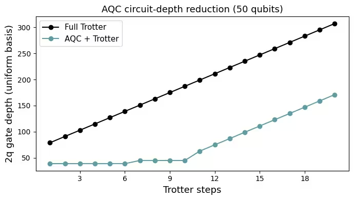
  At step 20 (uniform basis): Trotter 2q depth = 307, AQC+Trotter 2q depth = 171; 2q gates: Trotter = 3775, AQC+Trotter = 1913

Output of the previous code cell

Backend: ibm_fez
Transpiled 2q depth (deepest, ISA on ibm_fez): 105 (2q gates: 2574)
Job ID: d8v39vhropqc738biotg

Output of the previous code cell

Результати на апаратному забезпеченні відтворюють ключові риси двоспінонового континууму: інтенсивність розсіювання зосереджена поблизу антиферомагнітного хвильового вектора $q = \pi$ при низькій енергії та обмежена знизу синусоїдальною дисперсією спінонів, з широким континуумом спектральної ваги над нею, а не єдиною різкою модою. Це та ж сама структура, виміряна методом непружного розсіювання нейтронів на KCuF $_3$ , і вона підтверджує весь робочий процес підготовки основного стану, збурення, стисненої за допомогою AQC еволюції Троттера та вимірювання з пом'якшенням похибок у масштабі 50 кубітів.

Наступні кроки

Якщо ця робота видалась тобі цікавою, тебе можуть зацікавити такі матеріали:

Рекомендації

Моделювання розсіювання нейтронів за допомогою безсерверного робочого процесу динаміки AQC + Троттер — супровідний туторіал, який запускає той самий експеримент через розгорнутий шаблон функції Qiskit Serverless
Lee et al., "Benchmarking quantum simulation with neutron-scattering experiments" (arXiv:2603.15608) — довідкова стаття, на якій базується цей туторіал
Методи пом'якшення та придушення похибок — DD, твірлінг Паулі та TREX, використані в апаратних експериментах
Наближена квантова компіляція для схем еволюції в часі — туторіал з AQC-Tensor
Документація AQC-Tensor

Результати навчання​

Передумови​

Теоретичні відомості​

Непружне розсіювання нейтронів і динамічний структурний фактор​

KCuF3_33​: канонічний магнетик Латтінжерівської рідини​

Що ми моделюємо і вимірюємо​

Робочий процес квантового моделювання​

Наближена квантова компіляція (AQC)​

Моделювання MPS​

Вимоги​

Налаштування​

Приклад для симулятора малого масштабу​

Крок 1: відображення класичних вхідних даних на квантову задачу​

Крок 2: оптимізація задачі для виконання на квантовому апаратному забезпеченні​

Крок 3: виконання за допомогою примітивів Qiskit​

Крок 4: постобробка та повернення результату в потрібному класичному форматі​

Виконання на апаратному забезпеченні великого масштабу​

Наступні кроки​

Результати навчання

Передумови

Теоретичні відомості

Непружне розсіювання нейтронів і динамічний структурний фактор

KCuF $_3$ : канонічний магнетик Латтінжерівської рідини

Що ми моделюємо і вимірюємо

Робочий процес квантового моделювання

Наближена квантова компіляція (AQC)

Моделювання MPS

Вимоги

Налаштування

Приклад для симулятора малого масштабу

Крок 1: відображення класичних вхідних даних на квантову задачу

Крок 2: оптимізація задачі для виконання на квантовому апаратному забезпеченні

Крок 3: виконання за допомогою примітивів Qiskit

Крок 4: постобробка та повернення результату в потрібному класичному форматі

Виконання на апаратному забезпеченні великого масштабу

Наступні кроки