Квантова наближена багатокритеріальна оптимізація

Орієнтовний час використання: 10 хвилин на процесорі Heron r2 (ПРИМІТКА: це лише оцінка. Твій час виконання може відрізнятися.)

Результати навчання

Цей туторіал розв'язує задачу оптимізації портфеля з обмеженою кардинальністю: за умови володіння рівно $K$ активами збалансувати цілі щодо ризику, дохідності та диверсифікації, щоб знайти множину оптимальних портфелів.

Після проходження цього туторіалу ти зможеш зрозуміти:

• Як виразити задачу вибору портфеля з трьома конкуруючими цілями — низький ризик, висока дохідність і добра диверсифікація — як задачу квантової оптимізації.

• Як одна схема QAOA, пройдена по набору вагових коефіцієнтів цілей, прокладає фронт Парето оптимальних компромісних портфелів.

• Як мікшер XY утримує пошук усередині підпростору «вибрати рівно K активів», так що штрафний доданок не потрібен, а допустимість забезпечується постселекцією виміряних бітових рядків.

• Як навчити кути схеми за допомогою симулятора на матричних добутках станів у масштабі, надто великому для точної оптимізації, слідуючи Kotil et al. (arXiv:2503.22797).

Передумови

Рекомендується, щоб ти був знайомий із:

• Робочим процесом шаблонів Qiskit (відображення, оптимізація, виконання, постобробка).

• Основами QAOA.

Передісторія

Керівник портфеля рідко оптимізує одне число. Він хоче, щоб дохідність була високою, ризик (дисперсія цієї дохідності) — низьким, а активи були розподілені між секторами, щоб портфель не був надмірно прив'язаний до якоїсь однієї частини ринку. Ці цілі суперечать одна одній: активи з найвищою дохідністю часто найволатильніші, а концентрація в одному «гарячому» секторі шкодить диверсифікації.

Єдиного «найкращого» портфеля не існує. Натомість є фронт Парето: множина портфелів, для яких не можна покращити одну ціль, не поступившись іншою. Наша мета — відобразити цей фронт, щоб особа, яка ухвалює рішення, могла обрати бажаний компроміс.

Ми формулюємо задачу як вибір рівно $K$ активів із $N$ (кожен актив або входить, або ні — один кубіт на актив). Три гамільтоніани кодують три цілі. Ми комбінуємо їх із вагами $c$, що лежать на симплексі (їхня сума дорівнює одиниці), а семплер QAOA повертає добрі портфелі для кожного вибору ваг. Зміна ваг змінює відносну важливість ризику порівняно з дохідністю та диверсифікацією, а об'єднання всіх вибраних портфелів прокладає фронт Парето.

Спочатку ми пройдемо весь робочий процес на невеликому прикладі з восьми активів, який можна перевірити перебором, а потім запустимо той самий метод на екземплярі з 40 активів, розрахованому на квантове обладнання.

Цей туторіал навчає робочому процесу (відображення, навчання кутів, вибірка з обмеженнями та постобробка Парето), а не демонструє квантову перевагу. У масштабі з 40 активів, що використовується тут, рівномірна випадкова вибірка працює приблизно так само добре, як семплер QAOA, і ми явно показуємо це порівняння.

Вимоги

Перш ніж починати цей туторіал, переконайся, що встановлено таке:

• Qiskit SDK v2.0 або новіший із підтримкою візуалізації

• Qiskit Runtime v0.22 або новіший (pip install qiskit-ibm-runtime)

• Qiskit Aer (pip install qiskit-aer)

• Адон Qiskit Optimization mapper (pip install qiskit-addon-opt-mapper) і конвеєр навчання QAOA, закріплений на тегу v0.1.0: pip install "git+https://github.com/qiskit-community/qaoa_training_pipeline.git@v0.1.0"

• moocore для обчислень фронту Парето та гіперобсягу (pip install moocore)

Налаштування

Імпортуй бібліотеки, що використовуються протягом туторіалу, і зафіксуй випадкове зерно для відтворюваності.

# Added by doQumentation — installs the packages this notebook needs if they are missing
import importlib.util

_needed = {"matplotlib": "matplotlib", "moocore": "moocore", "numpy": "numpy", "qaoa_training_pipeline": "qaoa-training-pipeline", "qiskit": "qiskit", "qiskit_addon_opt_mapper": "qiskit-addon-opt-mapper", "qiskit_aer": "qiskit-aer", "qiskit_ibm_runtime": "qiskit-ibm-runtime", "scipy": "scipy"}
_missing = [pip for module, pip in _needed.items()
            if importlib.util.find_spec(module) is None]
# One at a time, so a package that fails to install does not block the others
for _pip in _missing:
    %pip install -q {_pip}
if not _missing:
    print("\u2713 All required packages are installed")

import numpy as np
import matplotlib.pyplot as plt
from math import comb
from moocore import hypervolume, filter_dominated, is_nondominated

from qiskit import QuantumCircuit
from qiskit.circuit import ParameterVector
from qiskit.circuit.library import qaoa_ansatz
from qiskit.quantum_info import SparsePauliOp
from qiskit.transpiler import generate_preset_pass_manager
from qiskit_aer.primitives import SamplerV2 as AerSampler
from qiskit_addon_opt_mapper.problems import OptimizationProblem
from qaoa_training_pipeline.training import ScipyTrainer
from qaoa_training_pipeline.evaluation import (
    StatevectorEvaluator,
    MPSAerEvaluator,
)

np.random.seed(42)
sampler = AerSampler(seed=42)  # local simulator for the small-scale example
print("Setup complete.")

Setup complete.

Приклад на симуляторі невеликого масштабу

Ми починаємо з восьми активів із шести секторів і вибираємо рівно $K=4$ з них. Маючи лише вісім активів, ми отримуємо лише $\binom{8}{4}=70$ допустимих портфелів, тож пізніше можемо звірити квантовий результат із вичерпним пошуком.

Крок 1: Відображення класичних вхідних даних на квантову задачу

Кожен актив — це один кубіт; бітовий рядок на кшталт 10110010 — це портфель (одиниці — активи, якими ми володіємо). Нам потрібні три складники: ринкові дані, три цільові гамільтоніани та схема, яка пропонує лише портфелі з рівно $K$ активами.

# --- Small-scale universe: 8 assets across 6 sectors ---
tickers = ["AAPL", "XOM", "JPM", "JNJ", "KO", "AMT", "AMZN", "SLB"]
sectors = [
    "Tech",
    "Energy",
    "Finance",
    "Health",
    "Staples",
    "REIT",
    "Tech",
    "Energy",
]
n_assets = len(tickers)
K = 4  # choose exactly K assets
n_obj = 3  # risk, return, diversification

# Annualized expected returns
mu = np.array([0.28, 0.12, 0.22, 0.05, 0.08, 0.10, 0.32, 0.15])

# Annualized covariance matrix (the "risk" model)
sigma = np.array(
    [
        [0.070, 0.010, 0.020, 0.008, 0.005, 0.012, 0.045, 0.011],
        [0.010, 0.065, 0.015, 0.006, 0.004, 0.008, 0.009, 0.050],
        [0.020, 0.015, 0.055, 0.010, 0.007, 0.015, 0.018, 0.014],
        [0.008, 0.006, 0.010, 0.030, 0.012, 0.009, 0.007, 0.005],
        [0.005, 0.004, 0.007, 0.012, 0.025, 0.006, 0.004, 0.003],
        [0.012, 0.008, 0.015, 0.009, 0.006, 0.045, 0.011, 0.007],
        [0.045, 0.009, 0.018, 0.007, 0.004, 0.011, 0.085, 0.010],
        [0.011, 0.050, 0.014, 0.005, 0.003, 0.007, 0.010, 0.072],
    ]
)

# Diversification score: number of cross-sector pairs in the portfolio.
# D[i,j] = 0.5 when assets i and j are in different sectors, so x^T D x counts
# the cross-sector pairs. More cross-sector pairs = better diversified.
D = np.array(
    [
        [1.0 if sectors[i] != sectors[j] else 0.0 for j in range(n_assets)]
        for i in range(n_assets)
    ]
)
np.fill_diagonal(D, 0.0)
D = D / 2

print(f"{n_assets} assets, choose K={K}, {n_obj} objectives")
for t, s, m in zip(tickers, sectors, mu):
    print(f"  {t:5s} ({s:8s})  expected return {m:5.0%}")

8 assets, choose K=4, 3 objectives
  AAPL  (Tech    )  expected return   28%
  XOM   (Energy  )  expected return   12%
  JPM   (Finance )  expected return   22%
  JNJ   (Health  )  expected return    5%
  KO    (Staples )  expected return    8%
  AMT   (REIT    )  expected return   10%
  AMZN  (Tech    )  expected return   32%
  SLB   (Energy  )  expected return   15%

# Each objective becomes a Hamiltonian whose lowest-energy bitstrings are the
# best portfolios for that objective. The opt-mapper turns a plain
# min/max problem over binary variables into the equivalent Ising operator.
def build_risk_hamiltonian(sigma, n):
    """Minimize portfolio variance x^T sigma x  (quadratic -> ZZ terms)."""
    prob = OptimizationProblem("risk")
    prob.binary_var_list(n)
    prob.minimize(quadratic=sigma)
    op, _ = prob.to_ising()
    return op.simplify()

def build_return_hamiltonian(mu, n):
    """Maximize expected return mu . x  (linear -> Z terms)."""
    prob = OptimizationProblem("return")
    prob.binary_var_list(n)
    prob.maximize(linear=mu)
    op, _ = prob.to_ising()
    return op.simplify()

def build_diversity_hamiltonian(D, n):
    """Maximize cross-sector pairs x^T D x  (quadratic -> ZZ terms)."""
    prob = OptimizationProblem("diversity")
    prob.binary_var_list(n)
    prob.maximize(quadratic=D)
    op, _ = prob.to_ising()
    return op.simplify()

H_risk = build_risk_hamiltonian(sigma, n_assets)
H_return = build_return_hamiltonian(mu, n_assets)
H_diversity = build_diversity_hamiltonian(D, n_assets)
cost_ops = [H_risk, H_return, H_diversity]

for name, op in zip(["risk", "return", "diversity"], cost_ops):
    print(f"H_{name:10s}: {op.size} Pauli terms")

H_risk      : 36 Pauli terms
H_return    : 8 Pauli terms
H_diversity : 34 Pauli terms

Забезпечення «рівно K активів» без штрафу. Поширений прийом — додати штрафний доданок, що карає портфелі неправильного розміру, але він зв'язує кожен кубіт із кожним іншим, що призводить до значно глибших схем після транспіляції. Натомість ми використовуємо мікшер XY, який переміщує стан QAOA лише між бітовими рядками з однаковою вагою Геммінга. Якщо ми починаємо зі стану, у якому вже вибрано $K$ активів, кожен портфель, який досліджує схема, також має рівно $K$ активів. Обмеження закладено в структуру схеми, а не забезпечується штрафним доданком.

Початковий стан ми готуємо дешево: повертаємо кожен кубіт так, щоб він був «увімкнений» з імовірністю $K/N$. Обмежений результатами з $K$ активами, він відтворює ідеальний рівновагий стан (Дікке), тож ми просто залишаємо виміряні бітові рядки, що мають рівно $K$ одиниць, — крок, який називається постселекцією.

def xy_mixer(n):
    """Line XY mixer: couples neighboring qubits with XX+YY. Conserves the number
    of selected assets (Hamming weight), so cardinality is preserved automatically.
    Using a line (not a full ring) keeps the circuit shallow and hardware-friendly."""
    terms = [
        (pauli, [i, i + 1], 1) for i in range(n - 1) for pauli in ("XX", "YY")
    ]
    return SparsePauliOp.from_sparse_list(terms, n)

def product_init(n, k):
    """Cheap initial state: each qubit rotated so P(selected) = k/n. Zero two-qubit
    gates. Post-selecting its weight-k outcomes reproduces the ideal Dicke state."""
    qc = QuantumCircuit(n)
    theta = 2 * np.arcsin(np.sqrt(k / n))
    for q in range(n):
        qc.ry(theta, q)
    return qc

# Combine the three objectives with weights c (bound later, at sampling time).
p_layers = 1
c = ParameterVector("c", n_obj)
# Negate the objective so the sampling phase separator matches the sign the angles
# were trained under (the trainer maximizes the negated sum); binding below keeps +gamma.
combined_cost_op = sum(
    -c[k] * H_k for k, H_k in enumerate(cost_ops)
).simplify()

ansatz = qaoa_ansatz(
    combined_cost_op,
    reps=p_layers,
    initial_state=product_init(n_assets, K),
    mixer_operator=xy_mixer(n_assets),
)
ansatz.measure_all()

betas = [p for p in ansatz.parameters if p.name.startswith("β")]
gammas = [p for p in ansatz.parameters if p.name.startswith("γ")]
print(f"Qubits: {ansatz.num_qubits} | QAOA layers: {p_layers}")
print(
    f"Tunable angles: {len(betas)} beta + {len(gammas)} gamma, plus {n_obj} objective weights"
)

Qubits: 8 | QAOA layers: 1
Tunable angles: 1 beta + 1 gamma, plus 3 objective weights

Крок 2: Оптимізація задачі для виконання на квантовому обладнанні

Перед запуском абстрактна схема транспілюється в рідні для обладнання вентилі. У цьому невеликому масштабі ми лише переглядаємо вартість: яка глибина схеми та скільки двокубітних вентилів вона використовує? (Двокубітні вентилі — головне джерело шуму на реальних пристроях.)

# Bind dummy angle values so we can transpile and measure the circuit's size.
dummy = {p: 0.1 for p in ansatz.parameters}
test_pm = generate_preset_pass_manager(optimization_level=1)
test_qc = test_pm.run(ansatz.assign_parameters(dummy))

print(f"Circuit depth          : {test_qc.depth()}")
print(
    f"Two-qubit gate depth   : {test_qc.depth(lambda x: len(x.qubits) > 1)}"
)
print(f"Two-qubit gate count   : {test_qc.num_nonlocal_gates()}")

Circuit depth          : 25
Two-qubit gate depth   : 23
Two-qubit gate count   : 42

Крок 3: Виконання за допомогою примітивів Qiskit

Два етапи. Спочатку ми один раз навчаємо кути QAOA з рівними вагами цілей за допомогою точного симулятора вектора стану, щоб знайти добрі значення $\beta,\gamma$. Потім ми проходимо по багатьох векторах ваг на симплексі та вибираємо схему для кожного, збираючи портфелі-кандидати. Оскільки між проходами змінюються лише ваги цілей (а не навчені кути), усі вектори ваг подаються в одному пакетному завданні.

# Train the angles with equal objective weights.
# The trainer maximizes energy, so we negate the (to-be-minimized) objective sum.
training_op = sum(-1.0 / n_obj * H_k for H_k in cost_ops).simplify()

# Linear-ramp initialization (Sack and Serbyn, arXiv:2101.05742)
dt = 0.75
grid = np.arange(1, p_layers + 1) - 0.5
init_params = np.concatenate((1 - grid * dt / p_layers, grid * dt / p_layers))

trainer = ScipyTrainer(
    StatevectorEvaluator(), minimize_args={"options": {"maxiter": 300}}
)
print("Training QAOA angles (exact statevector)...")
result_train = trainer.train(
    cost_op=training_op,
    mixer=xy_mixer(n_assets),
    initial_state=product_init(n_assets, K),
    params0=init_params,
)
opt = result_train["optimized_params"]
opt_betas, opt_gammas = opt[:p_layers], opt[p_layers:]
print(f"Trained beta : {opt_betas}")
print(f"Trained gamma: {opt_gammas}")

Training QAOA angles (exact statevector)...
Trained beta : [3.329186967386619]
Trained gamma: [3.4449804324291033]

def random_uniform_simplex(n_samples, n_obj=3):
    """n_samples weight vectors spread uniformly over the (n_obj-1)-simplex."""
    s = np.zeros((n_samples, n_obj + 1))
    s[:, 1:-1] = np.random.rand(n_samples, n_obj - 1)
    s[:, -1] = 1
    s = np.sort(s, axis=1)
    return np.diff(s, axis=1)

# Bind the trained angles, leaving the objective weights c free for the sweep.
param_map = {betas[i]: opt_betas[i] for i in range(p_layers)}
param_map.update({gammas[i]: opt_gammas[i] for i in range(p_layers)})
ansatz_bound = ansatz.assign_parameters(param_map)

n_samples, shots = 200, 500
c_vecs = random_uniform_simplex(n_samples, n_obj)

print(f"Sampling {n_samples} weight vectors x {shots} shots...")
result = sampler.run([(ansatz_bound, c_vecs)], shots=shots).result()

# Collect every distinct bitstring seen across all weight vectors.
all_bitstrings = set()
for s in range(n_samples):
    for bs in result[0].data.meas.get_counts(s):
        # get_counts is little-endian; reverse so bit i = asset i
        all_bitstrings.add(bs.replace(" ", "")[::-1])
print(f"Distinct portfolios sampled: {len(all_bitstrings)}")

Sampling 200 weight vectors x 500 shots...
Distinct portfolios sampled: 256

Крок 4: Постобробка та повернення результату в потрібному класичному форматі

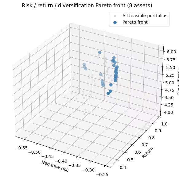
Ми залишаємо лише допустимі портфелі (рівно $K$ активів із кроку постселекції), оцінюємо кожен за всіма трьома цілями та виділяємо фронт Парето: портфелі, які не перевершені одночасно за всіма цілями. Гіперобсяг — це одне число, що підсумовує, скільки простору цілей домінує фронт, і чим більше, тим краще.

Зі 100 000 шотів лише по 256 бітових рядках цей запуск бачить кожен із 70 допустимих портфелів, тож за такого розміру це фактично перевірка перебором того, що конвеєр налаштовано правильно, а не доказ того, що QAOA знайшов фронт.

def evaluate_portfolio(bitstring, sigma, mu, D):
    """Score one portfolio on all three objectives (all framed as 'bigger is better')."""
    x = np.array([int(b) for b in bitstring])
    # negative risk, return, diversification (cross-sector pairs)
    return np.array([-(x @ sigma @ x), x @ mu, x @ D @ x])

# Post-select feasible portfolios, then score them.
feasible = [bs for bs in all_bitstrings if bs.count("1") == K]
fis = np.array([evaluate_portfolio(bs, sigma, mu, D) for bs in feasible])

pareto_front = filter_dominated(fis, maximise=True)
ref_point = fis.min(axis=0)
qmoo_hv = hypervolume(fis, ref=ref_point, maximise=True)

print(
    f"Feasible portfolios found : {len(feasible)} of {comb(n_assets, K)} possible"
)
print(f"Pareto-front portfolios   : {len(pareto_front)}")
print(f"Hypervolume               : {qmoo_hv:.4f}")

Feasible portfolios found : 70 of 70 possible
Pareto-front portfolios   : 26
Hypervolume               : 0.2487

fig = plt.figure(figsize=(8, 6))
ax = fig.add_subplot(111, projection="3d")
ax.scatter(
    fis[:, 0],
    fis[:, 1],
    fis[:, 2],
    c="lightgray",
    s=12,
    label="All feasible portfolios",
)
ax.scatter(
    pareto_front[:, 0],
    pareto_front[:, 1],
    pareto_front[:, 2],
    c="steelblue",
    s=45,
    label="Pareto front",
)
ax.set_xlabel("Negative risk")
ax.set_ylabel("Return")
ax.set_zlabel("Diversification")
ax.set_title("Risk / return / diversification Pareto front (8 assets)")
ax.legend()
plt.tight_layout()
plt.show()

Приклад на обладнанні великого масштабу

Тепер той самий робочий процес на 40 активах (8 секторів × 5), з вибором $K=6$. Сорок кубітів — надто багато для точної симуляції (вектор стану з $2^{40}$ амплітуд), тож кути не можна оптимізувати так, як для восьми активів, а щільна схема була б надто глибокою для сучасного обладнання. $\binom{40}{6} \approx 3.8$ млн допустимих портфелів усе ще достатньо мало, щоб перелічити їх класично, що ми використовуємо наприкінці як точний еталон. Кілька речей змінюються, і більше нічого в методі не змінюється:

1. Навчай кути за допомогою симулятора на матричних добутках станів (MPS), а не точного вектора стану. Слідуючи першоджерелу (Kotil et al.), ми фіксуємо рівні значення ваг цілей, оптимізуємо єдині β, γ на симуляторі MPS і повторно використовуємо їх для кожного вектора ваг у проході. (Ми навчаємо в тому розмірі, в якому запускаємо — без перенесення кутів із малого розміру на великий.)

2. Розрідь модель ризику, щоб вона вмістилася на обладнанні. Повна коваріація зв'язує всі 780 пар активів. Ми залишаємо лише найсильніші, найдешевші для маршрутизації зв'язки за допомогою усічення QAP з урахуванням важливості і зв'язуємо кожен сектор легким кільцем для доданка диверсифікації. Це зберігає змістовність цілей і тримає схему в розмірі, придатному для обладнання.

3. Тримай схему неглибокою та оцінюй чесно. Маршрутизація стохастична, тому ми транспілюємо з кількома зернами й залишаємо найменш глибоку (і квантовий час не витрачається). Портфелі завжди оцінюються за справжніми, повними цілями. Розрідження лише формує схему, а не те, як оцінюються портфелі.

Навіщо усічення QAP?

Залишення найбільших за модулем зв'язків кожного активу лише за величиною може призвести до схеми, яка розріджена, але все одно незручна для маршрутизації. Усічення QAP натомість залишає зв'язки, що є і великими, і фізично близькими на чипі, тож той самий бюджет вентилів дає менш глибоку, зручнішу для обладнання схему.

Крок 1: Відображення вхідних даних (розріджених для обладнання)

import csv
import urllib.request

# Download the committed market-data snapshot from the repo.
# --- 40-asset universe: 8 GICS sectors x 5 tickers (real market data) ---
# Load the committed market-data snapshot (real annualized returns and covariance).
# Values are stored at the precision used to train the shipped QAOA angles
# (mu: 3 dp, sigma: 4 dp), so the pre-trained parameters in instances/ stay exactly valid.

url = "https://raw.githubusercontent.com/Qiskit/documentation/main/datasets/tutorials/qmoo/market_data.csv"
urllib.request.urlretrieve(url, "market_data.csv")

with open("market_data.csv", newline="") as _f:
    _rows = list(csv.reader(_f))

# Covariance column order
_tickers_csv = _rows[0][2:]
# Asset tickers
tickers_40 = [r[0] for r in _rows[1:]]
# Annualized expected returns
mu_40 = np.array([float(r[1]) for r in _rows[1:]])
# Covariance (risk model)
sigma_40 = np.array([[float(v) for v in r[2:]] for r in _rows[1:]])

sectors_40 = [
    "Tech",
    "Tech",
    "Tech",
    "Tech",
    "Tech",
    "Energy",
    "Energy",
    "Energy",
    "Energy",
    "Energy",
    "Finance",
    "Finance",
    "Finance",
    "Finance",
    "Finance",
    "Health",
    "Health",
    "Health",
    "Health",
    "Health",
    "Staples",
    "Staples",
    "Staples",
    "Staples",
    "Staples",
    "Industrials",
    "Industrials",
    "Industrials",
    "Industrials",
    "Industrials",
    "Utilities",
    "Utilities",
    "Utilities",
    "Utilities",
    "Utilities",
    "REIT",
    "REIT",
    "REIT",
    "REIT",
    "REIT",
]
n_assets_40 = len(tickers_40)
K_40 = 6  # choose exactly K assets

sector_names_40 = list(dict.fromkeys(sectors_40))
sect_idx_40 = np.array([sector_names_40.index(s) for s in sectors_40])
# True cross-sector diversification matrix (used for scoring)
D_40 = np.array(
    [
        [
            0.5 if sectors_40[i] != sectors_40[j] else 0.0
            for j in range(n_assets_40)
        ]
        for i in range(n_assets_40)
    ]
)
np.fill_diagonal(D_40, 0.0)
print(
    f"{n_assets_40} assets, {len(sector_names_40)} sectors, choose K={K_40}"
)

40 assets, 8 sectors, choose K=6

# Sparsify the covariance so the risk circuit fits on hardware. A small diagonal
# shift (added after truncation) keeps the risk model positive semidefinite; at fixed
# K it adds the same constant to every portfolio, so it never changes the ranking.
# Importance-aware QAP truncation (Kotil et al. style): place the qubits on a line
# and use a Quadratic Assignment Problem to choose the layout that keeps the
# strongest covariance couplings within routing distance k of the swap network,
# then drop the rest. Unlike a fixed top-k cap, it keeps couplings that are both
# large AND cheap to route.
from scipy.optimize import quadratic_assignment as qap
from qiskit.transpiler.passes.routing.commuting_2q_gate_routing import (
    SwapStrategy,
)

# Truncation level: larger k keeps more couplings (deeper circuit)
k_truncate = 2
_dist = np.array(
    SwapStrategy.from_line(list(range(n_assets_40))).distance_matrix
)

def qap_truncate(Q, k):
    w = np.abs(Q.copy())
    np.fill_diagonal(w, 0.0)
    mask = (_dist <= k).astype(float)
    # Seed the QAP solver explicitly (by default it draws from NumPy's global
    # RNG, which SciPy is deprecating) so the truncation is reproducible.
    perm = qap(-w, mask, options={"rng": np.random.default_rng(42)}).col_ind
    keep = mask[np.ix_(perm, perm)]
    Qt = Q * keep
    np.fill_diagonal(Qt, np.diag(Q))
    return Qt

sigma_sparse = qap_truncate(sigma_40, k_truncate)
print(
    f"QAP truncation (k={k_truncate}): risk edges kept = "
    f"{(np.count_nonzero(sigma_sparse) - n_assets_40) // 2}"
)
ridge = max(0.0, -np.linalg.eigvalsh(sigma_sparse)[0]) + 1e-6
sigma_sparse = sigma_sparse + ridge * np.eye(n_assets_40)

# Diversity: couple each sector's assets in a ring (sparse stand-in for the
# same-sector pair count). Scoring still uses the true cross-sector matrix D_40.
def build_same_sector_hamiltonian(D_same, n):
    prob = OptimizationProblem("diversity_sparse")
    prob.binary_var_list(n)
    prob.minimize(quadratic=D_same)
    op, _ = prob.to_ising()
    return op.simplify()

D_ring = np.zeros((n_assets_40, n_assets_40))
for s in set(sect_idx_40):
    members = np.where(sect_idx_40 == s)[0]
    for k in range(len(members)):
        i, j = members[k], members[(k + 1) % len(members)]
        D_ring[i, j] = D_ring[j, i] = 0.5

H_risk_40 = build_risk_hamiltonian(sigma_sparse, n_assets_40)
H_return_40 = build_return_hamiltonian(mu_40, n_assets_40)
H_diversity_40 = build_same_sector_hamiltonian(D_ring, n_assets_40)
cost_ops_40 = [H_risk_40, H_return_40, H_diversity_40]
n_zz = sum(
    1 for p in sum(cost_ops_40).simplify().paulis if str(p).count("Z") == 2
)
print(
    f"Cost-layer interactions: {n_zz} (dense would be {n_assets_40*(n_assets_40-1)//2})"
)

QAP truncation (k=2): risk edges kept = 78
Cost-layer interactions: 102 (dense would be 780)

Кроки 2-3: навчання кутів, потім побудова та подання завдання для обладнання

Сорок кубітів — надто багато для точної оптимізації кутів, тому ми навчаємо єдині $\beta, \gamma$ на симуляторі на матричних добутках станів із рівними вагами цілей і повторно використовуємо їх у проході. Комірка нижче завантажує попередньо навчені значення з файлу. Навчений кут шару вартості малий ($\gamma \approx 0.32$), тож схема застосовує м'яке зміщення, а не різке проєктування.

import json
from qiskit_ibm_runtime import QiskitRuntimeService, SamplerV2

# Pre-trained angles loaded from a file (training is slow; QDC pattern).
# Set load_params_file = False to retrain in-notebook.
load_params_file = True
params_url = "https://raw.githubusercontent.com/Qiskit/documentation/main/datasets/tutorials/qmoo/qaoa_params.json"
params_path = "qaoa_params.json"
if load_params_file:
    urllib.request.urlretrieve(params_url, params_path)
    qaoa_params = json.load(open(params_path))
    p_layers_hw = qaoa_params["p_layers"]
    opt_betas_40, opt_gammas_40 = qaoa_params["betas"], qaoa_params["gammas"]
else:
    # Same workflow as the small-scale example: qaoa_training_pipeline's MPSAerEvaluator
    # evaluates the QAOA energy on Aer's MPS simulator and supports the XY mixer.
    # As in the small-scale example the trainer maximizes energy, so we negate the
    # (to-be-minimized) objective sum; the 1/n_obj scaling matches the equal-weight
    # point of the sweep, so the trained gamma transfers directly to the weighted circuits.
    p_layers_hw = 1
    training_op_40 = sum(-1.0 / n_obj * H_k for H_k in cost_ops_40).simplify()

    dt = 0.75
    grid = np.arange(1, p_layers_hw + 1) - 0.5
    init_params_40 = np.concatenate(
        (1 - grid * dt / p_layers_hw, grid * dt / p_layers_hw)
    )

    trainer_40 = ScipyTrainer(
        MPSAerEvaluator({"matrix_product_state_max_bond_dimension": 24}),
        minimize_args={"options": {"maxiter": 80}},
    )
    print("Training QAOA angles (MPS simulator)...")
    result_train_40 = trainer_40.train(
        cost_op=training_op_40,
        mixer=xy_mixer(n_assets_40),
        initial_state=product_init(n_assets_40, K_40),
        params0=init_params_40,
    )
    opt_40 = result_train_40["optimized_params"]
    opt_betas_40, opt_gammas_40 = (
        list(opt_40[:p_layers_hw]),
        list(opt_40[p_layers_hw:]),
    )
    import os

    os.makedirs(os.path.dirname(params_path) or ".", exist_ok=True)
    json.dump(
        {
            "p_layers": p_layers_hw,
            "betas": opt_betas_40,
            "gammas": opt_gammas_40,
        },
        open(params_path, "w"),
        indent=2,
    )
    print(
        f"Trained angles saved to {params_path} (set load_params_file=True to reuse)."
    )

c40 = ParameterVector("c", n_obj)
# Negated to match the trained angles' sign, as in the small-scale cell; binding keeps +gamma.
combined_cost_op_40 = sum(
    -c40[k] * H_k for k, H_k in enumerate(cost_ops_40)
).simplify()
qc_40 = qaoa_ansatz(
    combined_cost_op_40,
    reps=p_layers_hw,
    initial_state=product_init(n_assets_40, K_40),
    mixer_operator=xy_mixer(n_assets_40),
)
qc_40.measure_all()
b40 = [p for p in qc_40.parameters if p.name.startswith("β")]
g40 = [p for p in qc_40.parameters if p.name.startswith("γ")]
pmap = {b40[i]: opt_betas_40[i] for i in range(p_layers_hw)}
pmap.update({g40[i]: opt_gammas_40[i] for i in range(p_layers_hw)})
ansatz_qc_40 = qc_40.assign_parameters(pmap)

service = QiskitRuntimeService()

# only use Heron devices
backend = service.least_busy(min_num_qubits=156)

# SABRE routing is stochastic: different seeds give different depths. Transpilation
# is classical (it costs no QPU time), so we transpile many seeds and keep only the
# shallowest circuit -- a free reduction in two-qubit depth before anything is sent
# to hardware. Only this single best circuit is ever executed.
n_seeds = 24
best = None
depths = []
for seed in range(n_seeds):
    pm = generate_preset_pass_manager(
        optimization_level=3, backend=backend, seed_transpiler=seed
    )
    qc = pm.run(ansatz_qc_40)
    d2 = qc.depth(lambda x: len(x.qubits) > 1)
    depths.append(d2)
    if best is None or d2 < best[0]:
        best = (d2, seed, qc)
isa_qc = best[2]
sd = sorted(depths)
print(
    f"Backend: {backend.name} | {n_seeds} seeds | two-qubit depth "
    f"best/median/worst = {sd[0]}/{sd[len(sd)//2]}/{sd[-1]} (best seed {best[1]})"
)
print(
    f"Selected circuit -> two-qubit gates: {isa_qc.num_nonlocal_gates()}, "
    f"two-qubit depth: {isa_qc.depth(lambda x: len(x.qubits) > 1)}"
)

Backend: ibm_kingston | 24 seeds | two-qubit depth best/median/worst = 220/261/300 (best seed 22)
Selected circuit -> two-qubit gates: 787, two-qubit depth: 220

# Submit one batched job (job mode; a single batch needs no Session).
# Extra shots: noise lowers the post-selection yield
n_samples_40, shots_40 = 24, 1500
c_vecs_40 = random_uniform_simplex(n_samples_40, n_obj)
sampler_hw = SamplerV2(mode=backend)
# Tag hardware jobs for tracking
sampler_hw.options.environment.job_tags = ["TUT_QAMOO"]
# Seconds; guard against runaway jobs
sampler_hw.options.max_execution_time = 600

# The QAOA angles are already bound; only the objective weights c remain free.
# Assign each weight vector to get one concrete circuit per point on the simplex.
bound_circuits_40 = [
    isa_qc.assign_parameters({c40[k]: cv[k] for k in range(n_obj)})
    for cv in c_vecs_40
]
job_hw = sampler_hw.run([(qc,) for qc in bound_circuits_40], shots=shots_40)
print(
    f"Submitted to {backend.name}: job id {job_hw.job_id()} ({len(bound_circuits_40)} circuits)"
)

Submitted to ibm_kingston: job id darcaalvr3kc73einokg (24 circuits)

Крок 4: Постобробка у фронт Парето та зчитування оптимальних портфелів

result_hw = job_hw.result()

# Post-select feasible portfolios (exactly K assets), score on the TRUE objectives.
feasible_40 = set()
for s in range(n_samples_40):
    for bs in result_hw[s].data.meas.get_counts():
        # get_counts is little-endian; reverse so bit i = asset i
        bs = bs.replace(" ", "")[::-1]
        if bs.count("1") == K_40:
            feasible_40.add(bs)

def score_40(P):
    """Score portfolios given as an (n, K) array of asset indices.

    Returns an (n, 3) array of [negative risk, return, diversification], all framed
    as 'bigger is better'. This is the single definition of the true objectives,
    used for the hardware samples, the exact enumeration, and the random baseline.
    Looping over the K x K index pairs keeps memory O(n) even for millions of rows.
    """
    risk = np.zeros(len(P))
    div = np.zeros(len(P))
    for a in range(P.shape[1]):
        for b in range(P.shape[1]):
            risk += sigma_40[P[:, a], P[:, b]]
            div += D_40[P[:, a], P[:, b]]
    return np.column_stack([-risk, mu_40[P].sum(1), div])

def evaluate_40(bs):
    """Score one bitstring (bit i = asset i) with score_40."""
    idx = np.flatnonzero([b == "1" for b in bs])
    return score_40(idx[None, :])[0]

fis_40 = np.array([evaluate_40(bs) for bs in feasible_40])
pareto_40 = filter_dominated(fis_40, maximise=True)
print(f"Feasible portfolios collected : {len(feasible_40)}")
print(f"Pareto-front portfolios       : {len(pareto_40)}")

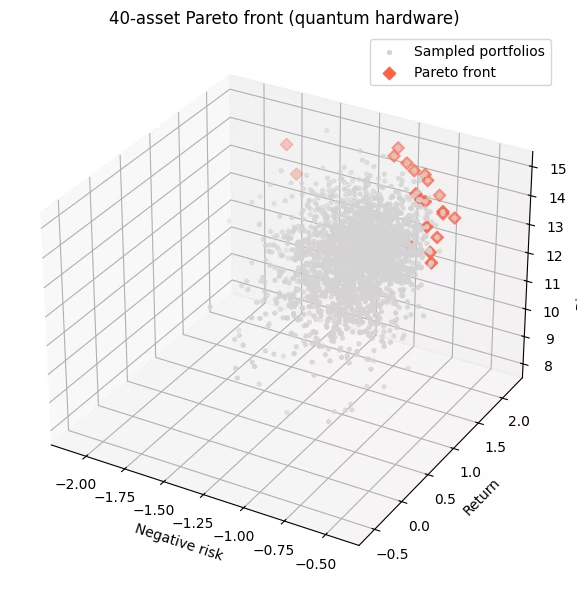
Feasible portfolios collected : 2359
Pareto-front portfolios       : 20

# --- Honest benchmark: QAOA and random vs the EXACT Pareto front ---
# 40 choose 6 = 3,838,380 feasible portfolios -- few enough to enumerate exactly, score
# every one on the TRUE objectives, and get the exact Pareto front. That front is an
# absolute ceiling, and its feasible nadir is a FIXED hypervolume reference point, so the
# numbers are comparable across runs instead of depending on what happened to be sampled.
import itertools

# Stream the combinations straight into an (n, K) index array, without first
# building millions of Python tuples.
combos = np.fromiter(
    itertools.chain.from_iterable(
        itertools.combinations(range(n_assets_40), K_40)
    ),
    dtype=np.int16,
).reshape(-1, K_40)
fis_exact = score_40(combos)
front_exact = filter_dominated(fis_exact, maximise=True)

# Fixed reference = worst value of each objective over ALL feasible portfolios (the nadir).
ref_fixed = fis_exact.min(axis=0)
# The hypervolume of a point set equals the hypervolume of its front.
hv_ceiling = hypervolume(front_exact, ref=ref_fixed, maximise=True)
hv_qaoa = hypervolume(fis_40, ref=ref_fixed, maximise=True)

def random_feasible_hv(n_draw, seed):
    """Hypervolume of n_draw uniformly-random feasible portfolios, same fixed reference."""
    rng = np.random.default_rng(seed)
    picks = set()
    while len(picks) < n_draw:
        picks.add(tuple(sorted(rng.choice(n_assets_40, K_40, replace=False))))
    P = np.array(list(picks))
    return hypervolume(score_40(P), ref=ref_fixed, maximise=True)

hv_rand = np.array(
    [random_feasible_hv(len(feasible_40), seed) for seed in range(20)]
)

print(f"Exact Pareto front            : {len(front_exact)} portfolios")
print(f"Hypervolume ceiling (optimum) : {hv_ceiling:.3f}")
print(
    f"QAOA (hardware)               : {100 * hv_qaoa / hv_ceiling:5.1f}% of optimum"
)
print(
    f"Random ({len(feasible_40)} draws, 20 seeds) : "
    f"{100 * hv_rand.mean() / hv_ceiling:5.1f}% +/- {100 * hv_rand.std() / hv_ceiling:.1f}% of optimum"
)

Exact Pareto front            : 61 portfolios
Hypervolume ceiling (optimum) : 64.211
QAOA (hardware)               :  85.5% of optimum
Random (2359 draws, 20 seeds) :  84.4% +/- 1.3% of optimum

За такого розміру задачі QAOA працює приблизно так само добре, як рівномірна випадкова вибірка. Обидва відновлюють значну частку гіперобсягу точного оптимуму, і жоден явно не випереджає. Такий результат очікуваний для одного неглибокого шару QAOA з сильно усіченим оператором вартості на шумному обладнанні; цінність цього прикладу — наскрізний багатокритеріальний робочий процес (відображення, навчання кутів, вибірка з обмеженнями та постобробка Парето), а не квантове прискорення. Зменшення розриву з оптимумом вимагало б глибших схем (більше шарів QAOA), м'якшого усічення або обладнання з меншим шумом.

# The best trade-offs found by the sampler: no other sampled portfolio beats these
# on every objective. They approximate the exact front computed above; a
# decision-maker picks the trade-off they prefer.
bs_list = list(feasible_40)
# Boolean mask over fis_40; keep_weakly=True also keeps portfolios whose
# objective values tie with a front point (what the strict filter would drop).
mask = is_nondominated(fis_40, maximise=True, keep_weakly=True)
front_bs = [b for b, m in zip(bs_list, mask) if m]
front_f = fis_40[mask]
order = np.argsort(-front_f[:, 1])  # show a span sorted by return
print(
    f"{mask.sum()} non-dominated sampled portfolios. A representative span:\n"
)
print(
    f"{'tickers held':40s} {'risk':>7s} {'return':>7s} {'cross-sector':>12s}"
)
for idx in order[:: max(1, len(order) // 12)]:
    held = [tickers_40[i] for i, b in enumerate(front_bs[idx]) if b == "1"]
    print(
        f"{', '.join(held):40s} {-front_f[idx,0]:7.3f} {front_f[idx,1]:7.2f} {int(front_f[idx,2]):12d}"
    )

fig = plt.figure(figsize=(8, 6))
ax = fig.add_subplot(111, projection="3d")
ax.scatter(
    fis_40[:, 0],
    fis_40[:, 1],
    fis_40[:, 2],
    c="lightgray",
    s=8,
    label="Sampled portfolios",
)
ax.scatter(
    pareto_40[:, 0],
    pareto_40[:, 1],
    pareto_40[:, 2],
    c="tomato",
    marker="D",
    s=40,
    label="Pareto front",
)
ax.set_xlabel("Negative risk")
ax.set_ylabel("Return")
ax.set_zlabel("Diversification")
ax.set_title("40-asset Pareto front (quantum hardware)")
ax.legend()
plt.tight_layout()
plt.show()

20 non-dominated sampled portfolios. A representative span:

tickers held                                risk  return cross-sector
AAPL, NVDA, XOM, GS, BLK, CAT              1.715    2.22           13
NVDA, GS, MS, PFE, CAT, PLD                1.772    2.20           14
NVDA, MS, PFE, WMT, CAT, DUK               1.040    2.14           15
NVDA, CVX, GS, JNJ, KO, WMT                0.737    2.01           14
NVDA, COP, GS, JNJ, WMT, EQIX              1.014    1.98           15
NVDA, ABT, WMT, CAT, AEP, EQIX             0.913    1.92           15
NVDA, CVX, WMT, RTX, D, EQIX               0.835    1.82           15
NVDA, XOM, GS, JNJ, DUK, EQIX              0.763    1.80           15
AAPL, NVDA, JNJ, KO, RTX, SO               0.621    1.71           14
NVDA, CVX, BLK, JNJ, RTX, AEP              0.719    1.71           15
NVDA, JNJ, KO, COST, RTX, AEP              0.545    1.69           14
NVDA, CVX, ABT, WMT, HON, AEP              0.702    1.43           15
AAPL, GS, JNJ, PEP, AEP, EQIX              0.645    1.34           15
MSFT, XOM, BLK, JNJ, CAT, SO               0.617    1.34           15
MSFT, KO, WMT, RTX, SO, SPG                0.526    1.29           14
MSFT, XOM, BLK, JNJ, WMT, DUK              0.483    1.25           15
MSFT, CVX, JNJ, RTX, DUK, D                0.482    1.02           14
MSFT, XOM, JNJ, KO, HON, EQIX              0.479    0.93           15
MSFT, JNJ, PG, KO, RTX, DUK                0.423    0.86           14
MSFT, XOM, JNJ, PEP, DUK, AMT              0.476    0.57           15

Наступні кроки

Рекомендації

Якщо цей туторіал здався тобі цікавим, розглянь таке:

• Заміни завантажені ринкові дані (market_data.csv) власними оцінками дохідності та коваріації з реальної історії цін.

• Збільш кількість шарів QAOA або навчи кути на 12–16 активах і перенеси їх, щоб наблизити фронт на обладнанні до оптимального.

• Прочитай Kotil et al., Quantum Approximate Multi-Objective Optimization (Nature Computational Science, 2025), дослідження max-cut, яке цей туторіал адаптує до портфелів.

Посилання

1. Kotil et al., "Quantum Approximate Multi-Objective Optimization," Nature Computational Science (2025). arXiv:2503.22797

2. S. H. Sack and M. Serbyn, "Quantum annealing initialization of the quantum approximate optimization algorithm," Quantum 5, 491 (2021). arXiv:2101.05742